2 Framework. We can think of the process of time-critical rendering of massive data as a parallel and progressive stream from back to front as shown in figure 2.
Scalable Isosurface Visualization of Massive Datasets on COTS� Clusters Xiaoyu Zhangy
Chandrajit Bajajy
William Blankez
Donald Fusselly
y
z
Department of Computer Science, Department of Electrical and Computer Engineering, University of Texas at Austin
Abstract Our scalable isosurface visualization solution on a COTS cluster is an end-to-end parallel and progressive platform, from the initial data access to the final display. In this paper we focus on the back end scalability by introducing a fully parallel and out-of-core isosurface extraction algorithm. It partitions the volume data according to its workload spectrum for load balancing and creates an I/O-optimal external interval tree to minimize the number of I/O operations of loading large data from disk. It achieves scalability by using both parallel processing and parallel disks. Interactive browsing of extracted isosurfaces is made possible by using parallel isosurface extraction and rendering in conjunction with a new specialized piece of image compositing hardware called Metabuffer. We also describe an isosurface compression scheme that is efficient for isosurface transmission. Keywords: Parallel Rendering, Metabuffer, Multi-resolution, Progressive mesh, Parallel and Out-of-core Isocontouring
1 Introduction and Related Works Today’s real time visualization applications increasingly are dealing with larger and larger data streams. In order to find the critical areas of interest within these datasets and understand the underlying physics, it is necessary that the application allows the user to navigate quickly and easily around the object space to explore different views. Given a Scalar Field, w( ), defined over a d-dimensional d ), we often visualize the data by bounded volume mesh ( rendering (d 1)-dimensional surfaces satisfying w( ) =const. This visualization technique is popularly known as Isocontouring and is widely used method for volume data visualization. Isocontour visualization for extremely large datasets poses challenging problems for both computation and rendering with guaranteed frame rates. To achieve scalable isosurface visualization in a time critical manner, we decompose the time-critical isosurface extraction and rendering into three pipeline stages2. First, isosurfaces are to be extracted efficiently from those large datasets. As the size of the input data increases, isocontouring algorithms need to be executed out-of-core and/or on parallel machines for both efficiency and data accessibility. Hansen and Hinker describe parallel methods for isosurface extraction on SIMD machines [17]. Ellsiepen describes a parallel isosurfacing method for FEM data by dynamically distributing working blocks to a number of connected workstations [13]. Shen, Hansen, Livnat and Johnson implement a parallel algorithm by partitioning load in the span space [31]. Parker et al. present a parallel isosurface rendering algorithm using ray tracing [26]. Chiang and Silva give an implementation of out-of-core isocontouring using the I/O optimal external interval tree on a single processor [7, 8]. Bajaj et al. use range
x2R
� Common of the shelf
x
x
partition to reduce the size of data that are loaded for given isocontour queries and balance the load within a range partition [3]. In this paper, we propose and implement a parallel and out-of-core isocontouring algorithm using parallel processors and parallel I/O, which would be fully scalable to arbitrarily large datasets. Second, The interactive aspect of the application demands that the scene is rendered quickly in order to provide responsive feedback to the user. At the same time, if an interesting area is found within the dataset, it is imperative that the application show the scene at the highest level of detail possible. In some cases, the detail allowed by a single high performance monitor may not be adequate for the resolution required. An even more common problem is that the dataset itself may be too large to store and render on a single machine. Many research groups have studied the problem of parallel rendering [6, 12, 18, 20, 22, 28–30]. Schneider analyzes the suitability of PCs for parallel rendering for four parallel polygon rendering scenarios: rendering of single and multiple frames on symmetric multiprocessors and clusters [30]. Samanta et al. discuss various load balancing schemes for a multi-projector rendering system driven by multiple PCs [29]. Heirich and Moll demonstrate how to build a scalable image composition system using off-the-shelf components [18]. In general, most parallel rendering methods can be classified based on where data is sorted from object-space to image-space [23]. In the sort-first approach, the display space is broken into a number of non-overlapping display regions, which can vary in size and shape. Because polygons are assigned to the rendering process before geometric processing, sort-first methods may suffer from load imbalance in both the geometric processing and rasterization if polygons are not evenly distributed across the screen partitions. Crocket [10] describes various considerations to build a parallel graphics library using the sort-first method. The Princeton University SHRIMP project [29] uses the sort-first approach to balance the load of multiple PC graphical workstations. The sort-last approach is also known as image composition. Each rendering process performs both geometric processing and rasterization independent of all other rendering processes. Local images rendered on the rendering processes are composited together to form the final image. The sort-last method makes the load balancing problem easier since screen space constraints are removed. However, compositing hardware is needed to combine the output of the various processors into a single correct picture. Such approaches have been used since the 60’s in single-display systems [15, 24, 25], and more recent work includes [14, 18]. Our solution to image compositing problem is the Metabuffer, whose architecture is shown in figure 1. This is a sort-last multidisplay image compositing system with several unique features such as multi-resolution and antialiasing [5]. A very similar project, though currently without stressing multi-resolution support, exists at Stanford University and is called Lightening-2 [19]. The Metabuffer hardware supports a scalable number of PCs and an independently scalable number of displays–there is no a priori cor-
respondence between the number of renderers and the number of displays to be used. It also allows any renderer to be responsible for any axis-aligned rectangular viewport within the global display space at each frame. Such viewports can be modified on a frameby-frame basis, can overlap the boundaries of display tiles and each other arbitrarily, and can vary in size up to the size of the global display space. Thus each machine in the network is given equal access to all parts of the display space, and the overall screen is treated as a uniform display space, that is, as though it were driven via a single, large framebuffer, hence the name Metabuffer. Because the viewports can vary in size, the system supports multi-resolution rendering, for instance allowing a single machine to render a background at low resolution while other machines render foreground objects at much higher resolution. Meta-Buffer
PC Workstations
out-of-core computation, parallel rendering and compression, it is possible to have a fully scalable system for interactive isocontour visualization across multiple isovalues and from different viewpoints. In this paper we focus on the back end parallel and out-ofcore isosurface extraction, leaving the details of progressive image composition using the Metabuffer and its performance result to a separate paper [5]. The rest of our paper is organized as follows: Section 2 briefly describes the architecture of our framework for scalable isosurface visualization. Section 3.1 gives the details of our parallel and out-of-core isocontouring algorithm. Section 3.2 provides the detail of our isosurface compression method and compares its results to that of another surface compression algorithm. Section 4 gives the performance of our parallel implementation on a COTS cluster.
2 Framework
Compositing Unit
A Rendering Engine
B
C
C
C
C
Frame Buffer
A
B
C
C
C
C
A
B
C
C
C
C
??? ??? ??? Display
Figure 1: Meta-Buffer architecture, where A represents rendering engine, B is on board frame buffer, C represents composing unit. Third, the extracted isosurface may need to be transmitted from the computational servers to the rendering servers via the network, if they do not coexist on the same machines. It may also need to be saved on disk for future studies. Compact representation of the isosurfaces should be used in order to meet the time limit of data transmission and to save disk space. One possible approach to this problem is to first extract the isosurface into triangular meshes and then apply to it one of the surface compression algorithms [4, 9, 11, 16, 32, 33]. Although it is conceptually simple, this method has several disadvantages. First the rendering servers have to wait until the computational servers finish both isosurface extraction and compression. The compression of the surface often takes a very long time, especially true for the very large surfaces extracted from large datasets, which contradicts the goal of using compression for real-time rendering. Furthermore, isosurfaces have the property that each vertex is an intersection point with one unique edge of the 3D volume. An algorithm designed specifically for isosurface may get better compression ratio. In this paper we describe an index and function value encoding scheme that compresses the isosurface and allows streaming the compressed data to the rendering servers incrementally either during the surface extraction or from cache on disk. We also show the method achieves better compression ratio than some general purpose surface compression algorithms. With all three aforementioned techniques combined, parallel and
We can think of the process of time-critical rendering of massive data as a parallel and progressive stream from back to front as shown in figure 2. Triangle streams are progressively generated by the back-end node that can take as input either a parallel triangle mesh hierarchy or hierarchical volume dataset, from which it extracts progressive isosurfaces. This stage is governed by the parallel and progressive triangle extraction algorithms. We will describe in detail our parallel triangle extraction algorithms in section 3.1. The triangle stream from the extraction node will be rendered by the middle parallel rendering servers. Each rendering server i s mapped to a viewport on the screen space. One very important problem in the parallel rendering is how to position those viewports and partition the mesh such that each rendering server has approximately an equal amount of work. All rendered images will then be composited by the Metabuffer to display on a multi-tiled screen. The process of compositing images from multiple rendering servers to multiple displays using the Metabuffer is called parallel image composition. Given the required frame rate, the refresh time between two frames needs to be shared among these three stages: triangle extraction, rendering and image composition. While the image composition time taken by the Metabuffer is constant, how much external time left in the frame interval determines what resolution of triangles will be extracted and rendered. Mesh Hierarchy
Parallel & Progressive Image Composition
Parallel & Progressive Rendering
Parallel & Progressive Triangle Extraction
Hierarchical Volume Dataset
Figure 2: Schematic drawing of the three stages of time-critical isosurface extraction and rendering process pipeline. Figure 3 illustrates the parallel end to end framework for scalable time-critical visualization. The parallel back-side provides multiresolution triangular meshes or isosurfaces extracted from the volume dataset to satisfy the time limit. Producing multi-resolution representation of the data at the back-side is essential for the time critical rendering of massive data. When the user changes viewing parameters frequently, coarser representations of the data are rendered in order to give the user responsive feedback. Only when the user chooses a certain viewing position and some interesting isovalue, the details of the progressive mesh or isocontour are streamed for rendering in order to produce higher resolution image. Due to the large size of the massive dataset, it is extremely time-consuming or even impossible for doing progressive mesh construction and isosurface extraction on single processor. In order to scale to very large
datasets, we use a computational back end consisting of both parallel processors and parallel disks. Although the rendering servers might be on the same set of machines as the triangle extraction processes, the progressive triangle mesh extraction processes can in general scale independently of the number of parallel rendering servers. To reduce the time of data transmission over the network, the extracted mesh is communicated to rendering servers in compressed format. Projector
Processor
...
Network
Cluster
Projector
MetaBuffer
Projector
Display Observer
Processor Rendering Server
Given the progressivity from the triangle extraction stage to final image composition stage in our framework and the fact that each stage is fully parallelizable, we achieve a truly scalable time critical rendering of large isosurfaces.
3 Algorithms In this section we will discuss in more detail about the parallel and out-of-core isocontouring algorithm and the isosurface compression algorithm mentioned in section 2 that enables the framework for scalable time-critical visualization of massive datasets. First we discuss the scalable algorithm of extracting progressive isosurfaces from large volume datasets.
Rendering Server Processor
Projector
IBM
Rendering Server
Parallel Front-Side
Mainframe
Parallel Back-side
Figure 3: System architecture for the scalable large data visualization framework, where back-side provides progressive mesh and front-side displays the mesh in a progressive fashion. One novel feature of the framework is the parallel rendering and image composition system that is able to render the given scene in the least latency. The parallel front-side is built around the Metabuffer [5], which is a custom hardware built from commodity PC components. The Metabuffer hardware provides several unique advantages to assist in rendering large surface in parallel. First, because the Metabuffer allows for the viewports rendered by each PC to be located anywhere within the total display space, it is possible to achieve a much higher degree of load balancing than if each PC were linked directly to a single display. Second, since the viewports may overlap, blocks that may happen to lie on the same Z-axis for a particular view can still be rendered on different processors. Allowing for workload divisions along the Z-axis in effect enhances the fineness of the granularity of dataset and allows for more even load balancing. Instead of being limited to a two dimensional space of data to partition, the application can work within three dimensions to parcel out portions of the surface to the rendering processors. Third, the Metabuffer allows the viewports to be of different resolutions. It is not always necessary to strictly divide the surface such that it can fit entirely within the area of a single, high resolution viewport. The multi-resolution capability of the Metabuffer also allows the progressive display of surface. It is possible to compute a good single resolution load balanced partition for a given viewing direction. However, when user shifts his view, some partitions can no longer fit within a single, high resolution viewport. It is not feasible to recompute the partition in a time critical environment. On the other hand, those viewports can be scaled to double, triple, or even higher multiples of the original size in order to cover their partition. Naturally, image quality is lost because the surface segments contained in those particular viewports are being displayed in lower resolutions, but the advantage is that the user will see no slowdown in exploring the dataset no matter how he or she changes the view. Instead of having to wait for the servers to reshuffle the triangles to conform to a new viewpoint, the scene is rendered immediately albeit in low resolution. Over time, for example when user fixes the viewpoint for a while, triangles can be shifted from server to server in order to reduce the maximum size of the viewport and thus increase its resolution. This increase in resolution over time is analogous to progressive display approaches in which a low quality image is displayed immediately with higher quality images appearing later.
3.1 Scalable Isosurface Extraction A scalable data analysis and visualization application must take data processing, I/O, network and rendering all into consideration. Specifically for the isocontour extraction of large volume data, it should have load balanced parallel computation for fast surface extraction, out-of-core computation to scale to datasets bigger than the size of total main memory, and parallel I/O to avoid the bottleneck of accessing massive data on disk. We can model such a system that combines parallel processing and parallel disk access with a model called the BSP-Disk model [27]. The BSP-Disk model consists of P interconnected processors, each of which may have a local memory and disk. The BSPDisk model combines the features of the BSP parallel computation model [34] and the PDM [35] parallel disk model. It is a distributed memory parallel computation model, while each processor can access its local disk in parallel. The BSP-Disk model very closely describes the characteristics of a PC cluster, where each node has its own CPU, local memory and local disk. The parameters of the BSP-Disk model are as follows:
� � � � � � � �
: Total number of atomic units of the problem.
N
: Total number of atomic units that can fit in the one processor’s main memory.
M
P
: Number of processors.
D
: Number of Disks.
B
: Number of atomic units that fits in one disk block.
A
: Time to read or write one disk block on the local disk.
L
: minimal synchronization time of the BSP model.
: gap parameter of the BSP model which characterizes the communication bandwidth.
g
In the case of large datasets, we have the design conditions M and M B . In contrast to the PDM model where a single processor has equal access to all parallel disks, the disks in the BSP-Disk model are associated to different processors as their local disks. One very important example is that every processor has one associated local disk (P = D), as for the case of a PC cluster. P processors can be assigned to every disk. Extra More generally D communication time is required when one processor needs to access the data on a remote disk. In the BSP-Disk model one disk block can be loaded from every disk into memory in one parallel I/O because each disk can be accessed independently. Thus up to D disk blocks can be read into main memory in one parallel I/O. In other words, the data access time is shared among the D disks. When external memory access in out-of-core computation is considered, the number of parallel I/O is a very important factor N > P
�
�
work work
x
a
y
value
work
b y
x
value
x
y
value
work span x x
value
y
Triangular Matrix in Span Space
y
value
Ideal Data Partition for 3 Processors
Figure 4: Optimal data partition for parallel isocontouring (two processor case) with the help of triangular matrix in span space.
for the total running time. The PDM model [35] uses the number of parallel I/Os as the primary performance measure of a external memory algorithm. The algorithm designed for the BSP-Disk model would consider all three parts of the time for a real parallel and out-of-core algorithm, local computation, local disk I/O and communication. Therefore the time of the isosurface extraction can be written as T = maxP (Tw + Tio + T ), where Tw is time for local computation, Tio is the time for local disk access and T is the time for communication. Tw and T are to be measured using the BSP model and Tio is measured as A Nd , where Nd is the number of parallel I/O operations. The objective of our isocontouring algorithm for large datasets is to speedup the computation by distributing the load to multiple processors, minimize the number of parallel I/Os, and minimize inter-processor communication (such as the remote disk accesses). These factors do not always play together for each other. We must make tradeoffs according to the real system parameters. To minimize the number of parallel I/O’s, we need to load only those portions of dataset that contribute to the final result, and distribute data to the disks such that data is loaded evenly from the D local disks. Minimizing the local computation time requires good load balance among the processors. Finally minimizing communication means minimal data redistribution and remote data access during computation. We choose the approach of static data partitioning that minimizes the communication during isocontour extraction because data communication is currently the least scalable factor when data size gets larger and new processors and disks can be easily added. The methods of allowing processors to dynamically steal data or work from remote disks are for future study. In order to achieve good performance for a static workload allocation method for parallel computation, data must be partitioned carefully such that each processor has approximately same amount of work. Furthermore data must be distributed among the D disks such that the number of parallel I/O is minimal. Fortunately the work load of isocontouring computation on a processor is proportional to the size of data it loads from its local disk. We use a data partition method similar to that in [3] to distribute the data according the contour spectrum [2]. The contour spectrum, as shown in figure 4, provides a work load histogram for different isovalue queries. We use the number of triangles in the isosurface as the Y axis of the contour spectrum. Figure 4 shows the ideal partitioning of the data in the case of three processors. In this ideal data partition, each processor does the same amount of work for every value of the parameter v . While [3] tries to break data into range
�
partitions that can each fit into main memory, we here partition the whole range of data according to the workload histogram. The partitioning of the whole range avoids the problem of data duplication among different range partitions. After data is partitioned, an I/Ooptimal interval tree [1] is built as index structure for the data on each disk in a way similar to [8]. The external memory interval tree has optimal O(log N + K ) I/O operations for stabbing queries, where K is the number of active cells. Cell is the minimum unit of the volume dataset. Function values are defined on the vertices of the cells and usually tri-linearly interpolated inside cell. Ideally we can use the granularity of cell for the data partition and build the external interval tree for all the cells. However as shown in [8], it is very storage inefficient to build an external index data structure using the unit of cell because of the high overhead of data duplication among cells. Instead we use the atomic unit of block, which is usually a 3D rectangular slab of adjacent cells. Although some extra cells maybe be loaded because of the larger granularity, block provides the possibility of tradeoff between disk space and I/O efficiency. In our implementation, we choose the size of block as the disk block size such that one block can be loaded in one I/O operation. Because we use a block as the unit of data partition and accessing, it is possible to extract isosurface progressively at different resolution to give user the basic shape of the surface with minimum delay. Figure 5 shows an isosurface (isovalue 1200) of the Male MRI data is extracted and rendered at three different resolutions. At the first stage of our algorithm, we partition the data among multiple computational nodes and build the external interval tree as the index structure for the blocks on each disk. Here we have assumed each node has one processor and associated local disk. The parallel and out-of-core isocontouring algorithm consists of following steps. 1. Break the data into blocks. At the start of the data distribution, there is an initial distribution of data among those disks, which is not load balanced for isosurface query. For example, we can just break the big volume into slabs and each disk contains one slab of the data. First we divide the dataset into blocks, each of which has the order of disk block size. With each block, we store all the information for doing isocontour extraction on the block, including the function values of all vertices of the block and the geometric information such as the dimensions, the origin and the span of the block. We also store the range interval of the block explicitly. We construct a triangular matrix in range space to help the data partition as shown in figure 4. One axis of the matrix represents the entire range of function values which is divided into a specified number of buckets. The second axis is the number of buckets that the range of a block spans. The minimum function value of a block and the number of buckets spanned by its range determine which matrix elements it belongs to. For instance, if a block has range [x; y ℄ and the bucket interval size is a, the ) (y x) block would belong to the [ (x min a ; a ℄ matrix element. Thus blocks falling into the same matrix element have similar span in the range space. We categorize the blocks according to which range space triangular matrix element it falls into.
d
ed
e
2. Redistribute the data blocks. The blocks falling into the same matrix element are then assigned equally to the processors. This process is repeated for all the matrix elements. At the beginning of redistribution, the processors broadcast to each other the number of blocks in the matrix element and the statistical information about the blocks. Then each processor run the same algorithm to determine to which processors it needs to send blocks and from which processors it will receive blocks. Here first we try to make each processor have
Figure 5: Isosurfaces for the Male MRI data (isovalue = 1200) are extracted and rendered at different resolutions and viewpoints, where the left surface has 24; 084 triangles, the center surface has 651; 234 triangles and the right surface has 6; 442; 810 triangles.
the same number of blocks of the matrix element. Further consideration is given to minimize the number of blocks to be communicated. 3. Build external interval tree as the search data structure. During the redistribution of blocks, every block assigned to one processor is given a unique ID and added to a single file that contains all the blocks assigned to the processor. Every block is stored from the disk block boundary and its location is easily decided from its ID. While the block is written to the block file, its range interval associated with its ID is stored in an interval file, which will be used to build the index structure to the data blocks. Because even the index structure may not fit into the main memory while the data size gets larger, we choose the external interval tree [1, 7] for the full scalability of our algorithm. 4. Isocontour extraction. Given an isovalue, we first query the external interval tree to find all blocks whose range intersects the isovalue. Such stabbing query on external interval tree is simple and I/O optimal [1]. The isosurface is then extracted from those intersected blocks. The surface can be extracted in compressed format, as we describe later. To give the user quick response, the extracted surface is streamed to the parallel rendering servers which may reside on the same machine. The rendered images from the parallel rendering engines are then composed by the Metabuffer. Because we use the block as the atomic unit of data distribution and accessing, the surface can be extracted at different resolution to meet the different time requirement. User can get a quick view of the shape of the isosurface before he can pick an interesting isovalue and study it in more detail. This algorithm provides a load balanced and fully out-of-core method for isocontour extraction, which would be scalable to arbitrary large dataset. The extracted surface are rendered by the parallel rendering servers and finally composited by the Metabuffer. The surface extraction process and rending process can be run in parallel. Figure 6 shows one isosurface extracted and rendered by eight processors. Because we have used the diagram of triangle numbers to determine the partition of dataset, each processor will generate approximately equal number of triangles and balance the load of rendering.
3.2 Isosurface Compression The isosurfaces extracted on the computational servers need to be rendered by the rendering servers and composited by the
Figure 6: An isosurface of visible male MRI data is extracted on eight parallel processors and rendered by eight parallel rendering servers, where the isovalue is 800 and there are total 9,128,798 triangles.
Metabuffer. The computational processes and rendering processes might not be present on the same machines. Therefore isosurfaces need to be transmitted from the back-end to rendering processes via the network. Furthermore we need to save and cache those large isosurfaces extracted from large dataset to examine them from different viewing directions. Compact representation of the isosurface should be used in the transmission in order to meet the time limit. We employ an edge index encoding method to compress the isosurface. Depending on the function values at its 8 vertices greater or less than the isovalue p, cell can have 28 = 256 different configurations, which can be further reduce to 15 distinct cases according to rotational symmetry and vertex complement [21]. We can easily derive the indices of cell edges intersected by the isosurface from the cell index and its configuration. Given function values on the two endpoints of the intersected edge, the point on this edge intersected by the isosurface can be computed. A vertex that is the end point of an edge intersected by the isosurface is called a relevant vertex. Hence the representation of the isosurface has been reduced as encoding configurations of intersected cells and function values on the relevant vertices. We further notice that cell configuration can be determined if we know which vertices of its 8 corners are relevant vertices. Here are the steps taken by the edge index compression algorithm. 1. For every vertex on a slice, we set a bit r = 1 if it is a relevant vertex, r = 0 otherwise. Similarly for each cell in a layer between two slices, we set a bit i = 1 if it is intersected by isosurface, i = 0 otherwise. 2. Encode the vertex bitmap of a slice using arithmetic coding.
a 18GB data disk, and an nVdia Geforce II graphics card. These machines are connected by 100Mb/s ethernet and Servernet II. Our tests use the 100Mb/s ethernet for communication. These machines run Linux (kernel 2.2.18) as the operating system and each disk block size is 4,096 bytes. We use several datasets of different size, shown in table 2, and different number of machines to test the performance of the algorithm. The three test datasets, whose size ranges are from 656M B Name Male MRI Male cryosection Female cryosection
Dimension 512 1800 1600
� 512 � 1252 � 1000 � 1878 � 1000 � 5186
Size 656MB 6.6GB 16.5GB
Table 2: Three test datasets. Figure 7: Speedup of isocontour extraction and rendering for two isovalues (800 and 1200) of the Male MRI data compared to the ideal case 3. Encode the function values on the relevant vertices of the slice using second-order difference of their quantized values and arithmetic coding. 4. Encode the cell bitmap of a layer using arithmetic coding. 5. Repeat upper steps until there are no more slices and layers. This method has yielded very good compression ratio to isosurface of regular 3D mesh compared to the general purpose triangular surface compression algorithms as shown in table 1, where the general algorithm is that of [4]. Furthermore, the edge index method has the advantage of incremental encoding and decoding because two slices and one layer are necessary in main memory at any time for the encoding and decoding processes. Thus both the compression and decompression of the isosurface using edge index encoding need very limited main memory and the reconstruction of the surface can start far before the whole surface transmission is finished. Furthermore the encoding of indices and function values is done during isosurface extraction, such that no post-extraction compression process is necessary. Model Hipip Foot Foot Engine Engine
Value
Data Type
Orig. Size
Gen. Alg.
Edge Index
0.0 600. 1500. 180. 89.
float u_short u_short u_char u_char
904,794 7,536,227 8,680,214 3,601,040 16,341,149
81,610 587,060 759,362 224,800 1,045,158
60,315 455,079 432,787 127,040 673,161
Table 1: Comparison of compressed isosurface sizes in bytes using edge index coding with a general surface compression algorithm. The general compression algorithm uses 8 bits for each coordinate per vertex. For unsigned short and char data type, we encode them directly using the predictive coder. Float values are normalized and quantized using 32 bits for the first point and 14 bits for difference.
4 Implementation and Results In this section we present some experimental results of the parallel and out-of-core isocontouring algorithm and the parallel visualization framework. Our primary interest in those tests is to show the scalability of our algorithms to the size of data set and the number of computers. Our implementation platform is a cluster of Compaq SP750 PC workstations, each of which has a 733MHZ Pentium III processor with 256M of Rambus memory, a 9GB system disk and
to more than 16GB , are all from the visible human project of the National Library of Medicine. Each of those datasets is too large for a single PC to handle in its main memory. While all those datasets are from medical imaging, our algorithm can be certainly applied to other types of data, for example those from large scale simulation. The first test data is the Male MRI dataset. The surface extracted on one machine is rendered by the same machine and the images are then composited according their z values. Every rendering server in this configuration has the viewport of the whole displaying space. It is a configuration that every rendering server renders at the same resolution. We measure its isosurface extraction and rendering time by using from one processor to 32 processors. Being able to run efficiently on a single processor demonstrates the out-of-core property of our method. Figure 7 shows the speedup of isosurface extraction and rendering for two typical isovalues 800 and 1200, corresponding to the skin and bone respectively, for the MRI dataset. Figure 8 shows the actual time of each processor for the isovalue 800 with different number of processors.
Figure 8: Time for extracting and rendering an isosurface (isovalue 800) from the Male MRI data with 1, 8, 16 and 32 processors. The slopes of the two speedup curves are very similar, which demonstrates the the isocontour extraction algorithm applies equally well to different isovalues. The contour spectrums of data partitioning for the cases of 8, 16 and 32 processors are shown in figure 9. The first row of figures show the diagrams of the triangle numbers extracted by each processor for the range of isovalue from 0 to 1900, where the curves of the real experimental result in solid thin lines are compared to the ideal case in thick dashed line. The second row of figures are the actual surface extraction and rendering time for the whole range of isovalues. The similarity of the two set of curves justifies our using of the spectrum of triangle numbers as work load diagram.
(a) Triangle distribution for 8 processors
(b) Triangle distribution for 16 processors
(c) Triangle distribution for 32 processors
(d) Isocontouring time for 8 processors
(e) Isocontouring time for 16 processors
(f) Isocontouring time for 32 processors
Figure 9: The histogram of data partitioning for the Male MRI data, where the thick dashed line represent the averaged ideal case.
We also test our implementation on the much larger Male cryosection and Female cryosection datasets. Because of the 2GB file size limit of Linux, we start at partitioning the Male cryosection data into 8 pieces and the Female cryosection data into 16 pieces. Figure 10 shows the time of isosurface extraction and rendering for the two datasets for two different isovalues 13000 and 29000. It gives very good speedup when the number of processors and disks increases. The sharp drop of computational time from 8 processors to 16 processors for the Male cryosection data and from 16 processors to 32 processors for the Female cryosection data is due to the better operating system disk cache performance for the smaller partitions. A very large isosurface ( 487; 635; 342 triangles) extracted from the Female cryosection data is shown in Figure 11. While the surface is noisy due to the dataset, it demonstrates the scalability of our system to very large data and very large surface.
5 Conclusion and Future Work In this paper we propose a scalable time-critical rendering framework of massive datastreams based around the Metabuffer image composition hardware.The time-critical rendering process can be thought of as a chain from parallel and progressive mesh generation, parallel rendering to parallel image composition. We describe in detail a scalable isocontouring algorithm by taking advantage of the parallel processors and parallel disks. It partitions the volume data according to its workload spectrum for load balancing and creates an I/O-optimal external interval tree to minimize the number of I/O operations of loading large data from disk. There are improvements necessary for real interactivity for very large datasets. There are also the remaining problems of introducing dynamic load balancing by replicating some data on different disks and accessing data from remote disks at runtime. It is an in-
Figure 10: Isosurface extraction and rendering time for the Male cryosection and Female cryosection data at two different isovalues( 13000 and 29000).
[8] C HIANG , Y.-J., S ILVA , C. T., AND S CHROEDER , W. J. Interactive out-of-core isosurface extraction. In Proceedings of the 9th Annual IEEE Conference on Visualization (VIS-98) (New York, Oct. 18–23 1998), ACM Press, pp. 167–174. [9] C HOW, M. M. Optimized geometry compression for realtime rendering. In Proceedings of IEEE Visualization ’97 (Phoenix, 1997), pp. 347–354. [10] C ROCKETT, T. W. Parallel rendering. Tech. rep., ICASE, 1995. [11] D EERING , M. Geometry compression. Computer Graphics (SIGGRAPH ’95 Proceedings) (1995), 13–20. [12] E LDRIDGE , M., I GEHY, H., AND H ANRAHAN , P. Pomegranate: A fully scalable graphics architecture. Computer Graphics (SIGGRAPH 2000 Proceedings) (2000), 443– 454. [13] E LLSIEPEN , P. Parallel isosurfacing in large unstructed datasets. In Visualization in Scientific Computing (1995), Springer-Verlag, pp. 9–23.
Figure 11: A isosurface(isovalue 29000) extracted from the Female cryosection data with 487; 635; 342 triangles
teresting problem to see how much improvement we can achieve by choosing the right replication factor and data distribution.
References [1] A RGE , L., AND V ITTER , J. S. Optimal interval management in external memory. In Proc. IEEE Foundations of Computer Science (1996), pp. 560–569. [2] BAJAJ , C., PASCUCCI , V., AND S CHIKORE, D. The contour spectrum. In Proceedings of the 1997 IEEE Visualization Conference (October 1997). [3] BAJAJ , C., PASCUCCI , V., T HOMPSON , D., AND Z HANG , X. Parallel acclerated isocontouring for out-of-core visualization. In Proceedings of IEEE Parallel Visualization and Graphics Symposium (October 1999), pp. 97–104. [4] BAJAJ , C., PASCUCCI , V., AND Z HUANG , G. Single resolution compression of arbitrary triangular meshes with prop erties. In IEEE Data Compression Conference (1999), pp. 247– 256.
[14] E YLES , J., M OLNAR , S., P OULTON , J., G REER , T., L AS TRA , A., E NGLAND , N., AND W ESTOVER , L. Pixelflow: The realization. In Proceedings of the Siggraph/Eurographics Workshop on Graphics Hardware (August 1997), pp. 57–68. [15] F USSELL , D. S., AND R ATHI , B. D. A vlsi-oriented architecture for real-time raster display of shaded polygons. In Graphics Interface ’82 (May 1982). [16] G UEZIEC , A., TAUBIN , G., L AZARUS , F., AND H ORN , W. Cutting and stitching: Efficient conversion of a non-manifold polygonal surface to a manifold. Tech. Rep. RC-20935, IBM T.J. Watson Research Center, 1997. [17] H ANSEN , C., AND H INKER , P. Massively parallel isosurface extraction. In Visualization ’92 (September 1992). [18] H EIRICH , A., AND M OLL , L. Scalable distributed visualization using off-the-shelf components. In Parallel Visualization and Graphics Symposium – 1999 (San Francisco, California, October 1999), J. Ahrens, A. Chalmers, and H.-W. Shen, Eds. [19] H UMPHREYS , G., B UCK , I., E LDRIDGE , M., AND H AN RAHAN , P. Distributed rendering for scalable displays. In Proceedings of Supercomputing 2000 (October 2000). [20] H UMPHREYS , G., AND H ANRAHAN , P. A distributed graphics system for large tiled displays. In Proceedings of IEEE Visualization Conference (1999), pp. 215–223. [21] L ORENSEN , W., AND C LINE , H. Marching cubes: A high resolution 3d surface construction algorithm. Computer Graphics 21, 4 (July 1987), 163–169.
[5] B LANKE , W. J., BAJAJ , C., F USSELL , D. S., AND Z HANG , X. The metabuffer: A scalable multiresolution multidisplay 3-d graphics system using commodity rendering engines. Tr2000-16, University of Texas at Austin, February 2000.
[22] M AJUMDER , A., H E , Z., T OWLES , H., AND W ELCH , G. Achieving color uniformity across multiprojector displays. In Proceedings of IEEE Visualization Conference (2000), pp. 117–124.
[6] C HEN , Y., C LARK , D., F INKELSTEIN, A., H OUSEL , T., AND L I , K. Automatic alignment of high resolution multiprojector displays using an un-calibrated camera. In Proceedings of IEEE Visualization Conference (2000), pp. 125–130.
[23] M OLNAR , S., C OX , M., E LLSWORTH , D., AND F UCHS , H. A sorting classification of parallel rendering. IEEE Computer Graphics and Applications 14, 4 (July 1994).
[7] C HIANG , Y., AND S ILVA , C. T. I/O optimal isosurface ex´ (Nov. 1997), R. Yagel and traction. In IEEE Visualization 97 H. Hagen, Eds., IEEE, pp. 293–300.
[24] M OLNAR , S. E. Combining z-buffer engines for higher-speed rendering. In Proceedings of the 1988 Eurographics Workshop on Graphics Hardware (1988), Eurographics Seminars, pp. 171–182.
[25] M OLNAR , S. E. Image composition architectures for realtime image generation. Phd dissertation, technical report tr91046, University of North Carolina, 1991. [26] PARKER , S., S HIRLEY, P., L IVNAT, Y., H ANSEN , C., AND S LOAN , P. Interactive ray tracing for isosurface rendering. In Visualization ’98 (October 1998). [27] R AMACHANDRAN , V. Class discussion, November 1999. [28] R ASKAR , R., B ROWN , M., YANG , R., C HEN , W., W ELCH , G., T OWLES , H., S EALES , B., AND F UCHS , H. Multiprojector displays using camera based registration. In Proceedings of IEEE Visualization Conference (1999), pp. 161– 168. [29] S AMANTA , R., Z HENG , J., F UNKHOUSER , T., L I , K., AND S INGH , J. P. Load balancing for multi-projector rendering systems. In SIGGRAPH/Eurographics Workshop on Graphics Hardware (August 1999). [30] S CHNEIDER , B.-O. Parallel rendering on pc workstations. In Parallel and Distributed Processing Techniques and Applications (July 1998), pp. 1281–1288. [31] S HEN , H., H ANSEN , C., L IVNAT, Y., AND J OHNSON , C. Isosurfacing in span space with utmost efficiency (issue). In Visualization ’96 (1996), pp. 287–294. [32] TAUBIN , G., AND ROSSIGNAC , J. Geometric compression through topological surgery. ACM Trans. Gr. 17, 2 (1996), 84–115. [33] T OUMA , C., AND G OTSMAN , C. Triangle mesh compression. In Proceedings of the 24th Conference on Graphics Interface (GI-98) (1998), W. Davis, K. Booth, and A. Fourier, Eds., Morgan Kaufmann Publishers, pp. 26–34. [34] VALIANT, L. G. A bridging model for parallel computation. Communications of the ACM 33 (1990), 103–111. [35] V ITTER , J. S. External memory algorithms and data structure. In DIMACS Series in Discrete Mathematics and Theoretical Computer S cience (1999).