Decentralized Monitoring of Distributed Anytime Algorithms Alan Carlin
Shlomo Zilberstein
Department of Computer Science University of Massachusetts Amherst, MA 01003
Department of Computer Science University of Massachusetts Amherst, MA 01003
[email protected]
ABSTRACT Anytime algorithms allow a system to trade solution quality for computation time. In previous work, monitoring techniques have been developed to allow agents to stop the computation at the “right” time so as to optimize a given time-dependent utility function. However, these results apply only to the single-agent case. In this paper we analyze the problems that arise when several agents solve components of a larger problem, each using an anytime algorithm. Monitoring in this case is more challenging as each agent is uncertain about the progress made so far by the others. We develop a formal framework for decentralized monitoring, establish the complexity of several interesting variants of the problem, and propose solution techniques for each one. Finally, we show that the framework can be applied to decentralized flow and planning problems.
Categories and Subject Descriptors I.2.8 [Problem Solving, Control Methods, and Search]
General Terms Algorithms, Performance
Keywords bounded rationality, meta-level control, Dec-MDP
1.
INTRODUCTION
Anytime algorithms are algorithms that improve their solution as a function of time, and can return an answer when interrupted [7]. When such algorithms are used, one must decide when to stop computing and use the current solution. Russell and Wefald describe the situation: “first, real agents have only finite computational power; second, they don’t have all the time in the world... Typically, the utility of an action will be a decreasing function of time.” [16]. Several works have studied the tradeoff of utility for time in applied settings including intelligent system design [10], problem solving and search [19], and planning [21]. Much of the work so far has focused on a single decision maker, whereas work on bounded rationality in group decision making has been relatively sparse [6, 13]. To some extent, any approximate reasoning framework could be viewed as a form of bounded rationality. But unless one can establish some constraints on decision qualCite as: Decentralized Monitoring of Distributed Anytime Algorithms, Alan Carlin and Shlomo Zilberstein, Proc. of 10th Int. Conf. on Autonomous Agents and Multiagent Systems (AAMAS 2011), Tumer, Yolum, Sonenberg and Stone (eds.), May, 2–6, 2011, Taipei, Taiwan, pp. XXX-XXX. c 2011, International Foundation for Autonomous Agents and Copyright Multiagent Systems (www.ifaamas.org). All rights reserved.
[email protected]
ity, such interpretations of bounded rationality are not very interesting. It seems more attractive to define bounded rationality as an optimization problem constrained by the availability of knowledge and computational resources. One successful approach is based on using decision-theoretic principles to monitor and control the base-level decision making procedure. It has been shown that this monitoring approach can be treated as a Markov Decision Process (MDP) and it can be solved optimally offline and used to optimize decision quality with negligible run-time overhead [9]. This approach to bounded rationality relies on optimal metareasoning [16]. That is, an agent is considered bounded rational if it monitors and controls its underlying decision making procedure optimally so as to maximize the comprehensive value of the decision. Additional formal approaches to bounded rationality have been proposed. For example, bounded optimality is based on a construction method that yields the best possible decision making program given a certain agent architecture [15]. The approach implies that a bounded rational agent will not be outperformed by any other agent running on the same architecture. This is a stronger guarantee than optimal metareasoning, but it is also harder to achieve. Extending these computational models of bounded rationality to multi-agent settings is hard. Even if one assumes that the agents collaborate with each other – as we do in this paper – there is an added layer of complication. There is uncertainty about the progress that each agent makes with its local problem solving process. Thus the metareasoning process inherently involves nontrivial coordination among the agents. One existing approach for meta-level coordination involves multiple agents that schedule a series of tasks [14]. As new tasks arrive, each agent must decide whether to deliberate on the new information and whether to negotiate with other agents about the new schedule. Each agent uses an MDP framework to reason about its deliberation process. The coordination across agents is handled by negotiation, not by the MDP policy. A more recent work uses Dec-MDPs for meta-level control, with reinforcement learning to assign radars to agents [5]. In this paper, we extend optimal metareasoning techniques to collaborative multiagent systems. We consider a decentralized setting, where multiple agents are solving components of a larger problem by running multiple anytime problem solving algorithms concurrently. The main challenge is for each individual agent to decide when to stop deliberating and start taking action based on its own partial information. In some settings, agents may be able to communicate and reach a better joint decision, but such communication may not be free. We propose a formal model to study these questions and show that decentralized monitoring of anytime computation can be reduced to the problem of solving decentralized MDP (Dec-MDP) [3].
2.
DECENTRALIZED MONITORING
We focus in this paper on a multiagent setting in which a group of agents is engaged in collaborative decision making. Each agent solves a component of the overall problem using an anytime algorithm – an algorithm that can be stopped at any time and provide an approximate solution to the problem. Solution quality increases with computation time according to some known probabilistic performance profile. The purpose of metareasoning is to monitor the progress of the anytime algorithms in a decentralized manner and decide when to stop deliberation. Definition 1. The decentralized monitoring problem (DMP) is defined by a tuple < Ag, Q, ~ q 0 , A, T, P, U, CL , CG > such that: • Ag is a set of agents. • Q is a set Q1 ×Q2 ...×Qn , where Qi is a set of discrete quality levels for agent i. At each step t, we denote the vector of agent qualities by ~ q t ∈ Q, or more simply by ~ q ∈ Q, whose components are qi ∈ Qi . Components of ~ q t are qualities for individual agents. We denote the quality for agent i at time t by qit . • ~ q 0 ∈ Q is a joint quality at the initial step, known to all agents. • A = {continue, stop, monitorL, monitorG} is a set of metalevel actions available to each agent. The actions monitorL and monitorG represent locally and global monitoring, respectively. • T is a finite horizon representing the maximum number of time steps in the problem. • Pi is the transition model for the “continue” action for agent i. We will use notation P with i implied by context. For all i, t ∈ {0..T − 2}, qit ∈ Qi , and qit+1 ∈ Qi , P (qit+1 |qit ) ∈ [0, 1]. Furthermore, Σqt+1 ∈Qi P (qit+1 |qit ) = 1. We assume i that the transitions of any two agents i and j are independent of each other, that is, P (qit+1 |qit , qjt ) = P (qit+1 |qit ). • U (~ q , t) : Q × T → < is a utility function that represents the value of solving the overall problem with quality vector ~ q at time t. • CL and CG are the costs of the local monitoring and global monitoring actions respectively. Each agent solves a component of the overall problem using an anytime algorithm. Unless a “stop” action is taken by one of the agents, all the agents continue to deliberate for up to T − 1 time steps. At each time step, agents decide which option to take, to continue, stop, or monitor globally or locally. If all the agents choose to continue, then the time step is incremented and solution quality transitions according to P . However, agents are unaware of the new quality state determined by the stochastic transition. If any agent chooses to “stop”, then all agents are instructed to cease computation before the next time step, and the utility U (~ q , t) of the current solution is taken as the final utility. If an agent chooses to monitor locally, then a cost of CL is subtracted from the utility (for each agent that chooses monitorL) and the agent becomes aware of its local quality at the current time step. If any agent chooses to monitor globally, a single cost of CG is subtracted from the utility and all agents become aware of all qualities at the time step. The time step is not incremented after a monitoring action. After an agent chooses to monitor, it must then choose whether to continue or stop, at the same time step. Agents are assumed to know the initial quality vector ~ q 0 . An agent has no knowledge about quality in later time steps, unless a
monitoring action is taken. The “monitorL” action monitors the local quality; when agent i takes the “monitorL” action at time t it obtains the value of qit . However, it still does not know any compot nent of ~ q−i . A “monitorG” action results in communication among all the agents, after which they all obtain the global quality ~ q t.
3.
LOCAL MONITORING
In this section, we examine the concept of local monitoring. That is, each agent must decide whether to continue its anytime computation, stop immediately, or monitor its progress at a cost CL , and then decide whether to continue or stop deliberation and initiate joint execution. The main result in this section shows that a DMP with local monitoring decisions can be solved by first converting the problem to a Transition Independent Dec-MDP. Although the termination decision may seem to imply transition dependence, the dependence is eliminated in the construction of Theorem 1.
3.1
Complexity of Local Monitoring
When CL = 0, each agent should choose to monitor locally on every step, since doing so is free. When CG = ∞, agents should never choose to monitor globally. The following lemma and theorem shows that even for the simpler case where CL = 0, CG = ∞, and the number of agents is fixed, the problem of finding a joint optimal policy is NP-complete. The termination decision alone, made by agents with local views of quality, is NP-hard. L EMMA 1. The problem of finding an optimal solution for a DMP with a fixed number of agents |Ag|, CL = 0 and CG = ∞ is NP-hard in the number of quality levels. P ROOF. A nearly identical problem to this special-case DMP with zero monitoring cost is the Team Decision Problem (TDP) in Tsitsiklis [22]. Unfortunately, unlike in the Team Decision Problem, three joint decisions of a two-agent DMP (when either agent stops, or they both do) contain the same utility. Therefore we proceed directly to the underlying Decentralized Detection problem upon which the complexity proof of TDP is established. We show that the NP-complete Decentralized Detection (DD) problem can be solved by a three step DMP. The following definition is provided in [22]. Decentralized Detection: Given finite sets Y1 , Y2 , a rational probability mass function p : Y1 × Y2 → Q, a partition {A0 , A1 } of Y1 × Y2 . The goal is to optimize J(γ1 , γ2 ) over the selection of γi : Yi → {0, 1}, i = 1, 2, where J(γ1 , γ2 ) is given by X p(y1 , y2 )γ1 (y1 )γ2 (y2 ) (y1 ,y2 )∈A0
+
X
p(y1 , y2 )(1 − γ1 (y1 )γ2 (y2 ))
(y1 ,y2 )∈A1
Decentralized detection can be polynomially reduced to a three step DMP with CL = 0. The first step is a known joint quality ~ q 0. We define a unique quality level at the second and third step for each yi ∈ Yi . We will denote the quality level representing yi by qyi . Transition probabilities to the second step are defined by the probability mass function, P (qi2 , qj2 ) = p(y1 , y2 ). Each agent then monitors (for zero cost) and is aware of its local quality. We model the decision of selecting γi = 1 as a decision by agent i to continue, and of selecting γi = 0 as a decision by agent i to terminate. To accomplish this, the DMP transition model transitions deterministically to a unique quality at step 3, for each quality of step 2 of each agent. Utility on step 3 is defined so that: 2 2 3 3 U (qyi , qyj , 2) = 0, U (qyi , qyj , 3) = 1 iff (yi , yj ) ∈ A0 , and 2 2 3 3 U (qyi , qyj , 2) = 1, U (qyi , qyj , 3) = 0 iff (yi , yj ) ∈ A1 .
to a transition independent Dec-MDP. Policies and policy-values for the DMP will correspond to policies and policy-values for the transition-independent Dec-MDP. The conversion is as follows: The state space S i for agent i are tuples < qi , t0 , t >, where qi is a quality level (drawn from Qi ), t0 is the time step at which that quality level was monitored, and t is the number of the current time step. We also define a terminal state for each agent. The action space for all agents is {terminate, continue, monitor}. The transitions consist of the following: when the action is to continue, t is merely incremented. When the action is to terminate, the agent transitions to the terminal state. Let PMDP (s0 |s, a) be the transition function of the Dec-MDP. Let t0 represent the time step when an agent last monitored. When the action is to monitor, we have ∀qi , qi0 ∈ Qi : Figure 1: An example of the state space for one of the agents, while running the Dec-MDP construction of Theorem 1. When the agent continues, only the current time is incremented. When the agent monitors, the agent stochastically transitions to a new quality state based on its performance profile. The current time increments and monitoring time is set to the current time. Not shown, when either agent terminates, the agents get a reward based on the expectation of utility over their performance profiles. It should be clear from this construction that an optimal continuation policy which maps qyi to a decision to continue or terminate, can be used to construct γ(yi ) in DD. To show that this DMP is in NP, we will reduce to a transition independent Decentralized MDP (Dec-MDP), a problem which was shown by Goldman and Zilberstein to be NP-complete [8]. In the Dec-MDP model, each agent has a local state space (denoted S i ) available, similar to a classic MDP. The vector of states, one for each agent, is referred to as the joint state. Each agent takes one action from a set of actions denoted Ai , and actions have stochastic effects which change the local state. The vector of actions, one per agent, is referred to as the joint action. Finally, agents receive a joint reward (denoted R(~s, ~a)) for taking a joint action from a joint state. Execution takes place sequentially, a joint action is taken from a joint state, a joint reward is received, and the process repeats. In a finite horizon problem, there are T repetitions, with T being the horizon of the problem. An agent’s Dec-MDP policy is a mapping from its history of states and actions to a plan for future actions, and is denoted πi . Each agent is aware of its own local state and local action, but not necessarily the states and actions of the other agents at run-time. It is aware, however, of the other agents’ policies which were formed at planning time. The Dec-MDP model enforces the rule that the joint state is jointly fully observable. That is, between the agents, the whole state can be observed at every step. In typical formulations of Dec-MDP, this means each agent is aware of its local state but not the state of the other agents. In a transition independent Dec-MDP, state transitions of each agent are fully independent of each other, no agent can have an effect another agent’s local state. The only dependency between the agents is with respect to joint reward. T HEOREM 1. The problem of finding an optimal solution for a DMP with a fixed number of agents, CL = k and CG = ∞ is NP-complete. NP-hardness follows from above, with k = 0 as a special case. To show NP-completeness, we show that the problem can be reduced
PMDP (< qi0 , t00 , t0 > | < qi , t0 , t >, monitor) = 0 if t0 6= t or t0 6= t0 . 0
PMDP (< qi0 , t00 , t0 > | < qi , t0 , t >, monitor) = P (qit |qit0 ) if t0 = t00 = t The Reward is defined as zero if all agents choose to continue, as −kC if k agents choose to monitor and none of the agents are in a terminal state, as U (~ q ) if one of the agents chooses to terminate and none of the agents are in a terminal state, and as zero if any agent is in a terminal state. This reduction is polynomial, as the number of agent states in the Dec-MDP is |Qi |T 2 and number of actions is 3. The representation is transition-independent, as the state of each agent does not affect the state of the other agents. Note that when one agent terminates, the other agents do not enter a terminal state, such a specification would violate transition independence. Rather, this notion, that no reward is accumulated once any agent has terminated, is captured by the reward function. No reward is received if any of the agents are in a terminal state. Since reward is only received when one of the agents enters the terminal state, reward is only received once, and the reward received by the Dec-MDP is the same as the utility received by the DMP. Figure 1 shows a visual representation of the Dec-MDP reduction from a DMP with local monitoring costs. State consists of a tuple consisting of a quality level, the time at which the quality was monitored, and the current time. The “continue” action in the first step increments the current time. The “monitor” action increments the monitoring time to the current time, and probabilistically transitions quality according to the transition probability of the DMP applied to multiple steps. An optimal policy for the Dec-MDP produces an optimal policy for the corresponding multi-agent anytime problem. Note that the uncertainty of quality present when an agent does not monitor is simulated in the MDP. Even though, in an MDP, an agent always knows its state, in this reduction the transition is not executed until the monitoring action is taken. Thus, even though an MDP has no local uncertainty, an agent does not “know” its quality until the monitor action is executed, and thus the local uncertainty of the multi-agent anytime problem is represented.
3.2 3.2.1
Solution Methods with Local Monitoring Greedy Solution
We first build a solution that adapts the single-agent approach of Hansen and Zilberstein to the multi-agent case [9]. The adaption considers the other agents to be a part of the environment, and thus we name it the Greedy approach. Greedy computation does not take into account the actions of the other agents, we will initiate a
greedy computation by assuming that the other agents always continue, and that they will never monitor or terminate. We will then build upon this solution to develop a nonmyopic solution. For ease of explanation, we will describe the algorithm from a single agent’s point of view. It should be assumed that each agent is executing this algorithm simultaneously. Each agent begins by forming a performance profile for the other agents. We will use the term P r as a probability function assuming only “continue” actions are taken, extending the transition model P over multiple steps. Furthermore we can derive performance profiles of multiple agents from the individual agents, using the independence of agent transitions. For example, in the two agent case we use P r(~ q ) as shorthand for P r(qi )P r(qj ). Definition 2. A dynamic local performance profile of an anytime algorithm, P ri (qi0 |qi , ∆t), denotes the probability of agent i getting a solution of quality q 0 by continuing the algorithm for time interval ∆t when the currently available solution has quality q. Definition 3. A greedy estimate of expected value of computation (MEVC) for agent i at time t is: X X M EV C(qit , t, t + ∆t) = q ~t q ~ t+∆t
q t+∆t |~ q t , ∆t)(U (~ q t+∆t , t + ∆t) − U (~ q t , t)) P r(~ q t |qit , t)P r(~ The first probability is the expectation of the current global state, given the local state, and the second probability is the chance of transition. Thus, MEVC is the difference between the expected utility level after continuing for ∆t more steps, versus the expected utility level at present. Both of these terms must be computed based on the performance profiles of the other agents, and thus the utilities are summed over all possible qualities achieved by the other agents. Cost of monitoring, CL , is not included in the above definition. An agent making a decision must subtract this quantity outside the MEVC term. For typical utility functions, the agent faces a choice as to whether to continue and achieve higher quality in a longer time, or to halt and receive the current quality with no additional time spent. A monitoring policy makes that decision. Definition 4. A monitoring policy Π(qi , t) for agent i is a mapping from time step t and local quality level qi to a decision whether to continue the algorithm or act on the currently available solution. It is possible to construct a stopping rule by creating and optimizing a value function for each agent. First, create a new local-agent value function Ui such that X t Ui (qi , t) = P r(~ q−i )U (< qi , ~ q−i >, t) t q ~−i
Next, create a value function using dynamic programming, one step at a time: 8 if d = stop: > > > > if d = continue: > >P > : P r(qit+∆t |qi )Vi (qi , t + ∆t) q t+∆t i
to determine the following policy: 8 if d = stop: > > > > if d = continue: > > >P : P r(qit+∆t |qit )Vi (qi , t + ∆t) q t+∆t i
q2t q2t q2t
q1t = 1 -2 5 -2
=1 =2 =3
q1t = 2 0 -3 -1
q1t = 3 -1 -1 1
Table 1: An example of a case where greedy termination policy produces a poor solution. Entries represent the expected utility of continuing for a step. where ∆t represents a single time step and d is a variable representing the decision. In the above, a stop action yields an expected utility over the qualities of the other agents. A continue action yields an expectation over joint qualities at future step t + ∆t. The above definitions exclude the option of monitoring (thus incurring the costs CL and CG ), the choices are merely whether to continue or act. Thus, we must define a cost-sensitive monitoring policy, which accounts for CL and CG . Definition 5. A cost-sensitive monitoring policy, Πi,c (qi , t), is a mapping from time step t, quality level qi , and monitoring cost c into a monitoring decision (∆t, m) such that ∆t represents the additional amount of time to allocate to the anytime algorithm, and m is a binary variable that represents whether to monitor at the end of this time allocation or to stop without monitoring. Thus, a cost-sensitive monitoring policy at each step chooses to either blindly continue, monitor, or terminate. It can be constructed using dynamic programming and the value function below. The agent chooses ∆t, how many steps to continue blindly, as well as whether to stop or monitor after. If it stops, it receives expected utility, if it monitors it achieves value with a penalty of CL . 8 if d = stop: > > >P > t+∆t t > |qi )Ui (qi , t + ∆t) > q t+∆t P r(qi < i
Vc (qi , t) = max d,∆t
> > > if d = monitor: > > > :P t+∆t P r(q t+∆t |q t )Vc (qi , t + ∆t) − CL i i q i
A greedy monitoring policy can thus be derived by applying dynamic programming over one agent. On initialization, such an algorithm assigns each quality level on the final step a value, based on its expected utility over possible qualities of the other agents. Then, working backwards, it finds the value of the previous step, which is the maximum over: (1) the expected utility over the possible qualities of the other agents (if it chooses to stop). (2) The expected utility of continuing (if it chooses to continue). An algorithm to find a cost-sensitive monitoring policy can similarly find the expectation over each time step with and without monitoring, and compare the difference to the cost of monitoring.
3.2.2
Solution Methods: Modeling the Other Agents
The greedy solution can be improved upon to coordinate policies among all the agents. To illustrate, examine Table 1. Each entry represents the expected joint utility of continuing (thus increasing utility but also time cost), minus the expected utility of stopping. Assume all entries have equal probability and monitoring cost is zero, and that the value of stopping immediately is zero, and thus the values shown represent only the value of continuing. Agent 1 would greedily decide to continue if it is in state q1t = 1 only, as that is the only column whose summation is positive. Agent 2 would greedily continue if it has achieved quality q2t = 2, as that is the only row whose summation is positive. However, this would
mean that the agents continue from all joint quality levels which are in bold. The sum of these levels is negative, and the agents would do better by selecting to terminate all the time! We solve the DMP with CG = ∞ optimally by leveraging the bilinear program approach of Petrik and Zilberstein to solving transition independent Dec-MDPs [11]. We first convert the problem to the transition independent Dec-MDP model described above. We prune “impossible” state-actions, for example we prune states where t0 > t, as an agent can not have last monitored in the future. Then we convert the resulting problem into a bilinear program. A bilinear program can be described by the following objective function and constraints for the two-agent case (the framework is extensible beyond two agents if more agent-vectors are added): maximizex,y r1T x + xT Ry + r2 y subject to B1 x = α1 B2 y = α2 In our bilinear formulation of a DMP, each component of the vector x represents a joint state-action pair for the first agent (similarly, each component of y represents a state-action for the second agent). Following the construction of Theorem 1, each component of x represents a tuple < q1t0 , t0 , t, a > where q1 represents the last quality observed, t0 represents the time at which it was observed, t represents the current time, and a represents a continue, monitor, or terminate. Thus, the length of x is 3|Q1 |T 2 (assuming no pruning of impossible state-actions). Each entry represents the probability of that state and action occurring upon policy execution. The vectors r1 and r2 are non-zero for entries corresponding to state-actions that have non-zero local reward, for agents 1 and 2 respectively. We set these vectors to zero, indicating no local reward. The matrix R specifies joint rewards for joint actions, each entry corresponds to the joint reward of a single state-action in x and y. Thus, entries in R correspond to the joint utility U (~ q , t) of the row and column state, when any agent terminates. For entries where one agent monitors and the other agent terminates or continues, we adjust reward by −CL . Otherwise, joint reward is 0. For the constraints, α1 and α2 represent the initial state distributions, and B1 and B2 and correspond to the dual formation of the total expected reward MDP [12]. Intuitively, these constraints are very similar to the classic linear program formulation of maximum flow. Each constraint represents a state triple, and each constraint assures that the probability of transitioning to the state (which is the sum of state-actions that transition to it, weighted by their transition probabilities) matches the probability of taking the outgoing state-actions (which is the three state-actions corresponding to the state triple). A special case is the start quality, from which outgoing flow equals 1. Bilinear programs, like their linear counterparts, can be solved through methods in the literature [11]. These techniques are beyond the scope of this paper, one technique is to alternately fix x and y policies and solve for the other as a linear program. Although bilinear problems are NP-complete in general, in practice performance depends on the number of non-zero entries in R.
4.
GLOBAL MONITORING
Next, we examine the case where agents can communicate with each other (i.e., monitor globally). We will analyze the case where CL = 0 and CG = k, where k is a constant. For ease of description, we describe an on-line approach to communication. The online approach can be converted to an offline approach by anticipating all possible contingencies. We decide whether to communicate based on decision theory, agents compute Value of Information
(VoI), which is defined as follows: V oI = V ∗ (qi , t) − Vsync (qi , t) − CG where V ∗ represents the expected utility after monitoring, Vsync represents expected utility without monitoring (see below), and CG is cost of monitoring. In order to support the computation of Vsync and V ∗ , joint policies are produced at each communication point (or, for the offline algorithm, at all possible joint qualities). We define a helpful term V ∗ (~ q , t), (which decomposes into V ∗ (qi , ~ q−i , t) to more clearly identify the local agent), which is the value of a joint policy after communication and discovery of joint quality ~ q , as computed through the methodology of the last section with CL = 0. From the point of view of agent i, the value after communicating can then be viewed as an expectation over the quality of the other agents, based on their profiles. X P r(~ q−i , t)V ∗ (qi , ~ q−i , t) V ∗ (qi , t) = q ~−i
Similarly, Vsync is the value attached to quality qi and not communicating. This was computed as part of the local monitoring problem at the last point of communication, we use the subscript “sync” to remind us that Vsync (qi , t) depends on the policies created and qualities observed at the last point of communication. Non-myopic policies require each agent to make a decision as to whether to communicate or not at each step, resulting in the construction of a table resembling Table 1. We examined this table in a previous section when deciding whether to continue or stop. The table is used similarly for global monitoring, except the decision made by each agent is whether to communicate or not to communicate. Communication by either agent forces both agents to communicate and synchronize knowledge. Entries represent the joint state, and are incurred if either agent 1 decides to communicate from the row representing its quality, or agent 2 decides to communicate from the column representing its local knowledge. This problem, of deciding whether to communicate after each step, is NP-complete as well. We will show this by reducing to a transition independent Dec-MDP-Comm-Sync [2]. A Dec-MDPComm-Sync is a transition independent Dec-MDP with an additional property: After each step, agents can decide whether to communicate or not to communicate. If they do not communicate, agents continue onto the next step as with a typical transition independent Dec-MDP. If any agent selects to communicate, then all agents learn the global state. However, a joint cost of CG is assessed for performing the communication. Agents form joint plans at each time of communication. The portion of the joint plan formed by agent i after step t is denoted πit . T HEOREM 2. The DMP problem with CL = 0 and CG is a constant, is NP-complete. The proof of NP-hardness is similar to Lemma 1. To show that the problem is in NP, we can reduce the problem to that of finding the solution of a Dec-MDP-Comm-Sync. We create the following Dec-MDP-Comm-Sync from a DMP with CL = 0. • S i is the set Qi ∪ {fi } for agent i, where fi is a new “terminal” state for agent i. Q • Ai = {continue, terminate}; the joint action set is i Ai . • The transition model: PMDP (qit+1 |qit , continue) = P (qit+1 |qit ) PMDP (qit2 |qit1 , continue) = 0, ∀(t2 6= t1 + 1) PMDP (fi |qit , terminate) = 1, ∀qit ∈ S i
Problem (Local/Global) Max Flow Local RockSample Local Max Flow Global RockSample Global
Compile Time 3.5 .13 .04 .01
Solve Time 11.4 2.8 370 129
Table 2: Timing results in seconds. Compile time represents time to compile performance profile into bilinear problem, solve time measures time taken by the bilinear solver.
Figure 2: Expected Utility versus cost of time of non-myopic local monitoring of RockSample, for four different values of CL . For the four plots, from highest to lowest, the cost of monitoring was .5, 4, 7, and 10. • The reward function R(~ q t , ai ) = U (~ q , t) if ai = terminate for some i; 0 otherwise. • The reward function is 0 when any agent is in the final state. • The horizon T is the same as T from the DMP. • The cost of communication is CG . The reduction is polynomial as the number of states added is equal to T , and only one action is added. It is straightforward to verify that this reduction is polynomial. Having represented the DMP problem as a Dec-MDP-Comm-Sync, we can use solution techniques from the literature to solve the problem which make use of a VoI computation [2].
5.
EXPERIMENTS
We experimented on two decentralized decision problems involving anytime computation. First we profiled the RockSample domain, borrowed from the POMDP planning literature. In this planning problem, two rovers must each form a plan to sample rocks, maximizing the interesting samples. However, the location of the rocks are not known until runtime, and thus the plans can not be constructed until the rovers are deployed. We selected the HSVI algorithm for POMDPs as the planning tool [20]. HSVI is an anytime algorithm, the performance improves with time, its error bound is constructed and reported at runtime. Prior to runtime, the algorithm was simulated 10, 000 times on randomized RockSample problems, in order to find the performance profile. The resulting profile held 5 quality levels over 6 time steps. Second, we profiled the Ford Fulkerson maximum flow solution method. This motivating scenario involved a decentralized maximum flow problem where two entities must each solve a maximum flow problem in order to supply disparate goods to the customer. To estimate the transition model P in the DMP, we profiled performance of Ford Fulkerson through Monte Carlo simulation. The flow network was constructed randomly on each trial, with each edge capacity in the network drawn from a uniform distribution. Quality levels corresponded to regions containing equal-sized ranges of the current flow. From the simulation, a 3-dimensional probability table was created, with each layer of the table corresponding to the time, each row corresponding to a quality at that time, each column representing the quality at the next time step, and the entry representing the transition probability. We created software to compile a Decentralized MDP from the probability ma-
Quality 1 2 3 4 5
1 4 4 0 0 0
2 3 3 3 2 1
1 2 3 4 5
4 4 0 0 0
3 3 3 2 1
Agent 1 3 4 3 2 3 2 2 2 1 1 0 0 Agent 2 3 2 3 2 2 2 1 1 0 0
5 1 1 1 1 0
6 0 0 0 0 0
1 1 1 1 0
0 0 0 0 0
Table 3: Greedy Local Monitoring Policy for RockSample problem, C=2 K=8 trix, as described in the previous sections, and solved the resulting problem using a bilinear program. Three parameters of utility were varied with respect to each other: the reward for increasing quality, a linearly increasing cost of time, and the cost of monitoring. Experiments varied the latter two. For RockSample, the chosen utility function was 10(qi + qj − Kt), where t was time in seconds modulo 5, and we experimented with various values of K. For MaxFlow, utility was defined as 10(min(qi , qj ) − Kt), where min(qi , qj ) represents the lesser of the flows, t represents the time step, (defined for the profile as the time in seconds modulo 5), and K represents cost of time and was varied. For max flow there were 10 quality levels and 10 time steps for each agent. In this section we focus problems with costs of time which result in non-trivial continuation policies. When cost of time is very low with respect to quality increase, computation trivially always continues, and when cost of time is very high, computation stops immediately. When cost of time lies between these two extremes, the option of monitoring becomes interesting. Mean running time for the non-myopic variant of our algorithms is shown in Table 2. The MaxFlow problem was larger than the RockSample problem (containing more quality levels), thus consumed more time. The global formulations, as opposed to the local formulations, required a sub-problem formulation to precompute V ∗ at each communication point, and thus more time elapsed. Table 3 shows resulting policies of the Greedy algorithm for local monitoring on the RockSample problem. The policy is taken for K = 8 and C = 2, which we consider well motivated since the routine to report progress took approximately a quarter of a time step. Rows represent quality levels and columns represent the time step at which that quality level was observed. Entries represent the agent’s policy. Numbered entries represent to proceed that number of steps, and then terminate. For example, the entry in box (1, 1) represents that at step 1 with quality level 1, the Greedy policy proceeds 4 steps and then terminates. For this particular cost of time and cost of monitoring, the Greedy algorithm does not monitor at any step, although the Greedy algorithm did monitor for lower costs of monitoring. Also note that the Greedy algorithm is the same for agent 1 and agent 2, each is working off of the same profile and is
Quality 1 2 3 4 5
1 3M -
1 2 3 4 5
1M -
Agent 1 3 4 1M 1M 1M 1M 0 Agent 2 1M 2M 1M 2M 2M 1M 0 1M 0 2 -
5 2 2 2 1 0
6 0 0 0 0 0
1 1 1 1 0
0 0 0 0 0
(a) RockSample
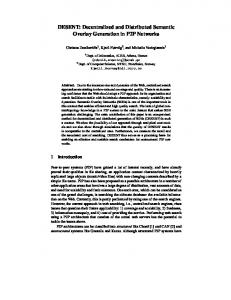
Table 4: Nonmyopic local monitoring policy for first agent C=2 K=8. In some cases, the bilinear program returned stochastic actions, where multiple state-actions corresponding to the same state had non-zero probability (the sum of the state-actions equaled one). In these cases, the tables show the most probable action for the state. not considering the policy of the other agent. Table 4 shows resulting policies of the Nonmyopic algorithm for the same local monitoring problem. Entries designated “xM” denote continuing for x steps and then monitoring. For instance, in the first step, the first agent will proceed for 3 steps and then monitor. The second agent, by contrast, will proceed one step and then monitor. In these policies, agents are more likely to stop at higher quality levels, and more likely to monitor at earlier points in time. Qualities that are impossible to achieve are reported with a “-”. The bilinear program only reports its policy for state-actions with probability above zero. For example, since agent 1 has a 100 percent chance of starting at quality level 1, and since the first step for agent 1 continues for three steps and then monitors, it is impossible to observe any quality level on the 2nd and 3rd steps. Figure 2 plots value versus the cost of time (K) for 4 different local costs of monitoring on the RockSample problem. For a constant cost of time, a higher cost of monitoring results in a lower quality solution. The drop off is monotonically decreasing and roughly linear, with higher cost of monitoring resulting in a more negative slope. This can be explained in context of the extremes of the graph. As one proceeds leftwards, cost of time is smaller, ultimately when it is small enough the agents should always continue (and, for instance when cost of time is zero, no monitoring decision is needed to verify this). As one proceeds rightwards, cost of time is larger, and when it is large enough the agents should stop on the first step (and again, no monitoring decision is required to verify this), achieving zero value. One can see that expected utility hits zero more quickly for the high cost of monitoring than the low cost of monitoring. Thus, the plots of all four monitoring costs intersect to the far left and the far right, but the zones where expected utility lies between those values is smallest when cost of monitoring is highest. Thus, higher cost of monitoring results in a more negative slope. Figure 3 (a) shows value of Global Monitoring as compared to Local Monitoring on RockSample for various time costs. Value with Global Monitoring is higher, due to the Cost of Local Monitoring being zero for the Global Monitoring case, as well as the ability of each agent to monitor the progress of other agents, thus coordinating further. Similarly, Figure 3 (b) summarizes experiments on MaxFlow. Nonmyopic monitoring outperforms myopic monitoring, and the global variant achieves higher performance. The RockSample domain proved more difficult to achieve higher scores, as the min function made it difficult to achieve value.
(b) MaxFlow Figure 3: Comparison of global monitoring, nonmyopic local monitoring, and local monitoring on RockSample and MaxFlow problems.
6.
RELATED WORK
The history of literature on anytime algorithms is rich in singleagent settings. We refer to [1, 6, 18] for recent overviews. Dean and Boddy used the term “anytime algorithm” in the 1980’s to describe a class of algorithms that "can be interrupted at any point during computation to return a result whose utility is a function of computation time" [7, 4]. They employed these algorithms in their work on time dependent planning and how to schedule deliberation. Horvitz, during the 1980’s as well, used decision theory to analyze "costs and benefits of applying alternative approximation procedures" to cases "where it is clear that there are insufficient computational resources to perform an analysis deemed as complete" [10]. Russell and Wefald used a discrete deliberation scheduling algorithm, which decides whether to deliberate or act based on expected value [16]. The work was implemented for search algorithms. Russell, Subramanian, and Parr utilized bounded optimality, which holds if a program produces a solution to a constrained optimization problem presented by the environment [15]. Work in artificial intelligence has produced several theories and architectures that can take into account the computational cost of decision making [7, 10, 15, 23, 24]. Zilberstein and Russell utilized performance profiles of algorithms in order to inform future anytime decisions [25]. The concept of performance profiles has been further explored in recent decision-theoretic approaches. Hansen and Zilberstein form a performance profile of an agent offline [9]. Then, based on this profile, a dynamic programming approach is used to make stopping decisions. The decisions use Bayesian reasoning based on the profiles in order to ascertain probability of future quality. Predictions of future quality are used to inform monitoring decisions, which are decisions whether to pause and monitor quality, or merely to continue. Similarly, Sandholm uses performance profiles to decide when to optimally terminate incomplete decision algorithms (algorithms which never finish if the answer is
N and may or may not finish if the answer is Y) on problems such as 3-SAT [17]. Termination decisions are based on the prior probability of an answer, on a utility model based on the utility of quality and time, and on the performance profiles. In the multi-agent realm, Raja and Lesser explore a framework for coordinating agents Meta-Level control [13, 14]. In these works a single agent or multiple agents schedule a series of tasks. At various points in time, new tasks arrive, and each agent must decide whether to deliberate on the new information and whether to negotiate with other agents about the new schedule. The authors use an MDP framework within agents to reason about deliberation and the coordination across agents is handled by negotiation. The recent approach of Cheng et al. uses reinforcement learning for meta-level control of weather radars, using Dec-MDPs [5].
7.
CONCLUSIONS AND FUTURE WORK
Anytime algorithms effectively gauge the trade-off between time and quality. Monitoring is an essential part of the process. Existing techniques from the literature weigh the trade-off between time, quality, and monitoring for the single-agent case. The complexity of the monitoring problem is known, and dynamic programming methods provide an efficient solution method. However, this paper shows that these techniques do not scale to the multi-agent case. In this paper, we took a decision-theoretic approach to the monitoring problem. We formalized the problem for the multi-agent case, and proved that there exist problems for both local and global monitoring which are NP-complete. We showed how the multi-agent monitoring problems can be compiled as special cases of Decentralized Markov Decision Processes, and thus solvers from the literature can produce efficient solutions. Future work lies in several directions. First, we will analyze and produce solutions for monitoring problems that are partially observable. We will also examine items like varying the monitoring cost. Second, we would like to examine cases with non-cooperative utility functions. Third, we will apply the methods to cases involving more than two agents. The latter will require modifications to the bilinear solver.
Acknowledgments Support for this work was provided in part by the National Science Foundation Grant IIS-0812149 and by the Air Force Office of Scientific Research Grant FA9550-08-1-0181.
8.
REFERENCES
[1] M. Anderson. A review of recent research in metareasoning and metalearning. AI Magazine, 28(1):7–16, 2007. [2] R. Becker, A. Carlin, V. Lesser, and S. Zilberstein. Analyzing myopic approaches for multi-agent communication. Computational Intelligence, 25(1):31–50, 2009. [3] D.S. Bernstein, R. Givan, N. Immerman, and S. Zilberstein The complexity of decentralized control of Markov decision processes. Mathematics of Operations Research, 27(1):819–840, 2002. [4] M. Boddy and T. Dean. Deliberation scheduling for problem solving in time-constrained environments. Artificial Intelligence, 67:244–285, 1994. [5] S. Cheng, A. Raja, and V. Lesser. Multiagent Meta-level Control for a Network of Weather Radars. In Proceedings of 2010 IEEE/WIC/ACM International Conference on Intelligent Agent Technology, 157-164, 2010. [6] M. Cox and A. Raja. Metareasoning: Thinking about thinking. Cambridge, MA: MIT Press.
[7] T. Dean and M. Boddy. An analysis of time-dependent planning. In Proceedings of the Seventh National Conference on Artificial Intelligence, 49–54, 1988. [8] C. Goldman and S. Zilberstein. Decentralized control of cooperative systems: Categorization and complexity analysis. Journal of Artificial Intelligence Research, 22:143–174, 2004. [9] E. Hansen and S. Zilberstein. Monitoring and control of anytime algorithms: A dynamic programming approach. Artificial Intelligence, 126(1-2):139–157, 2001. [10] E. Horvitz. Reasoning about beliefs and actions under computational resource constraints. In Proceedings of Third Workshop on Uncertainty in Artificial Intelligence, 429–444, 1987. [11] M. Petrik and S. Zilberstein. A bilinear approach for multiagent planning. Journal of Artificial Intelligence Research, 35:235–274, 2009. [12] M. Puterman. Markov decision processes, Discrete stochastic dynamic programming. John Wiley and Sons, Inc., 2005. [13] A. Raja and V. Lesser. Meta-level reasoning in deliberative agents. In Proceedings of the International Conference on Intelligent Agent Technology, 141–147, 2004. [14] A. Raja and V. Lesser. A framework for meta-level control in multi-agent systems. Autonomous Agents and Multi-Agent Systems, 15:147–196, 2007. [15] S. Russell, D. Subramanian, and R. Parr. Provably bounded optimal agents. In Proceedings of the Thirteenth International Joint Conference on Artificial Intelligence, 575–609, 1993. [16] S. Russell and E. Wefald. Principles of metareasoning. In Proceedings of the First International Conference on Principles of Knowledge Representation and Reasoning, 400–411, 1989. [17] T. Sandholm. Terminating decision algorithms optimally. In Proceedings of the International Conference on Principles and Practice of Constraint Programming, 2003. [18] M. Schut and M. Wooldridge. The control of reasoning in resource-bounded agents. Knowledge Engineering Review, 16(3):215–240, 2001. [19] H. Simon and J. Kadane. Optimal problem solving search: All or nothing solutions. Computer Science Technical Report CMU-CS-74-41, 1974. [20] T. Smith and R. Simmons. Heuristic search value iIteration for POMDPs. In Proceedings of the International Conference on Uncertainty in Artificial Intelligence, 520–527, 2004. [21] M. Stefik. Planning and meta-planning. Artificial Intelligence, 16(2):141–170, 1981. [22] J. Tsitsiklis and M. Athans. On the complexity of decentralized decision making and detection problems. IEEE Transactions on Automatic Control, 30(5):440–446, 1985. [23] M. P. Wellman. Formulation of Tradeoffs in Planning under Uncertainty. London: Pitman, 1990. [24] S. Zilberstein. Operational rationality through compilation of anytime algorithms. Ph.D. Dissertation, Computer Science Division, University of California, Berkeley, 1993. [25] S. Zilberstein and S. Russell. Optimal composition of real-time systems. Artificial Intelligence, 82(1-2):181–213, 1996. [26] S. Zilberstein. Metareasoning and bounded rationality. In M. Cox and A. Raja (Eds.), Metareasoning: Thinking about Thinking, MIT Press, forthcoming.