Safety in nuclear power plants requires reliable information concerning the state of the process. ... SDV3. knowledge-based: they rely on human expertise.
SELF-MONITORING DISTRIBUTED MONITORING SYSTEM FOR NUCLEAR POWER PLANTS (PRELIMINARY VERSION) Aldo Franco Dragoni Paolo Giorgini Istituto di Informatica, Università di Ancona, via Brecce Bianche, 60131, Ancona (Italy) Sensor data fusion and interpretation, sensor failure detection, isolation and identification are extremely important activities for the safety of a nuclear power plant. In particular, they become critical in case of conflicts among the data. If the monitored system’s description model is correct and its components work properly, then incompatibilities among data may only be attributed to temporary deterioration or permanent breakage of one or more sensors. This paper introduces and discusses three simple ideas: 1. classical “Model-Based Diagnosis” can be extended straightforwardly to encompass the sensors’ models into the system’s description in order to diagnose even their own faults 2. from the “log-file” of the diagnosed minimal conflicts among the sensors, one can draw interesting conclusion regarding their relative reliability (e.g., through Bayesian Conditioning) 3. the estimated reliability of the sensors is useful when assessing (e.g., through Dempster’s Rule of Combination) the actual state of the monitored physical system, even in cases of conflicting data. These ideas lead to the conception of a distributed monitoring system able to attach each sensor a statistically-evaluated relative reliability, which is especially useful for devices situated in dangerous zones or areas, difficult to reach inside huge and complex production plants.
1 INTRODUCTION Safety in nuclear power plants requires reliable information concerning the state of the process. Elaboration of data coming from the sensors of these complex plants is thus extremely important, and becomes critical when some sensors stop working properly. Failure detection, isolation and identification of sensor are indispensable activities for the monitoring system of a nuclear power plant. In recent years different approaches to the problem have been proposed. In [22], Kratz et al. presented a method based on the analytic redundancy for detecting and isolating sensor failures in a steam generator used in nuclear power plants. Keith and Belle in [23] developed signal validation software for application to nuclear power plant. Their system combines some previously
established fault detection methodologies as well as some newly developed modules. Again Keith, in [24] presented a study on the feasibility of using a feed-forward back propagation neural network in a signal fault detection capacity. The sensor data used in this study are taken from various subsystems within an operating nuclear power plant. More recently [25,26,27], Dorr and his colleague evaluated the contribution of analytic redundancy on the state estimation accuracy of linear systems. In these works, they carried out a comparative study of different methods of sensor fault detection using direct or indirect analytic redundancies on measurements obtained from a nuclear power plant. Normally, collected data are confronted with a theoretical model of the monitored process/phenomenon in order to specify its current state (in case of a control system) or to validate the theory (in case of a scientific experiment). Discrepancies between theoretical models and sensor data can be imputed either to the sensors or to the theory (or to both of them). We may distinguish between three basic cases: 1. at least one sensor did not adequately report the quantity it should have measured 2. the theoretical model is not (completely) applicable to the actual monitored system because: a) the (scientific) theory has to be refined (objective interpretation) b) the physical system is not working as it “should” (teleonomic interpretation) Case 1, often referred to as Sensor Data Validation (SDV), gained much interest in the last few years [1,2,3,4]. As illustrated in [5], methods can be distinguished into three categories: SDV1. data-based: they rely on statistical models obtained from observed data SDV2. model-based: they rely on an analytical model of the monitored system SDV3. knowledge-based: they rely on human expertise Case 2 has been deeply studied in Artificial Intelligence, both as a knowledge revision problem (BR for short, see [6] for an overview) and as a model-based diagnostic problem (MBD for short, see [7] for a survey). It seems evident to us that BR and MBD are dual problems. In the last decade, MBD moved from its theoretical foundation [8][9] to some practical applications (see for instance [10]). In MBD, diagnoses are found from discrepancies between observation and prediction. The intermediate step is the exhaustive generation of the “conflict sets” for the tuple (SD,COMPS,OBS), in which System Description and OBServations are sets of first order sentences, COMPonentS is a finite set of constants each one representing a component of the system [11]. A diagnosis is a subset of COMPS that covers all the conflict sets. A main problem with MBD is that each of its three fundamental steps, prediction, conflict recognition and candidate generation, exhibits a combinatorial explosion for large devices [12]. However, the worst problem with MBD is related to the case 2a before, i.e., the fact that it is at least difficult to find out a correct model for the system to diagnose. This paper does not deal with these problems: both of them will be cravenly avoided by imposing the relative simplicity of the apparatus to be controlled or diagnosed. Instead, this paper introduces, discusses and reports experimental results about the following three issues: 1. the problem of recognizing sensors’ faults can be approached entirely within the framework of MBD (section 2)
2. from the diagnostics of the sensors’ faults one can formulate interesting conclusions regarding the various sensors’ relative reliability (section 3) 3. from the estimated reliability of the sensors one can hypothesize the actual state of the monitored physical system even in cases of not-redundant and conflicting data (section 4). Normally, sensors come labeled with many important qualifications (accuracy, average life-time, ...) which are necessary to estimate their a priori current reliability. By “reliability” of a sensor we mean the “probability that the sensor is providing the correct measure,” whatever the term “correct” may signify. However, the actual current reliability of a sensor may be lesser than the “a priori” one due to unpredictable and/or unknown events that might have been occurred to it from its assembly to its current employment into the monitoring system. Of course, any sensor’s current conditions can be appraised through appropriate testing devices1. But, apart from the academic problem of infinite regression (which devices will test the testing devices, and so on, ...), a concrete question is that “testing” has its own costs. For instance, in the monitoring apparatus of an automatic production line, some optical sensors might have been altered after a temporary fault of the conditioning device that cleans the air from the pollution particles produced by the power generator. Since testing the sensors implies stopping the manufacturing process, other evidence about their possible deterioration would be appreciated. In the case of thermic sensors situated in proximity to kernel of a nuclear power plant, evidence about the wearing away of a limited number of sensors will drastically reduce the costs of maintenance. Issue 2 before suggests that such an evidence may come from the theoretical model of the monitored process/phenomenon and from the global datum provided by the distributed monitoring apparatus. The group of the sensors acts as a testing device for each one of its own members. Of course, this evaluation depends on the average reliability of all the sensors in the group (hence including the corrupted ones) and on the accuracy of the monitored entity’s model. In any case, these estimates will not be comparable (nor for quality neither for typology) with the evaluations made by specifically designed testing devices. Their point is that they do not interfere in any way with the manufacturing process, thus they have no expenses at all (apart from the fixed costs of a CPU, some data-acquisition boards and a mass storage device). A key idea with this distributed auto-estimate is that of “minimal conflicts”. Intuitively, if it has been detected a minimal conflict between the sensors A and B (by confronting the collected data with the theoretical model) and, subsequently, another minimal incompatibility is found involving B and C, then one may suppose more probable the deterioration of B than those of both, A and C. Dealing with probabilities, we do not want to reinvent the wheel since Bayesian Conditioning [13] (section 3) seems an appropriate tool to accomplish the task. Basically, the new reliability of a sensor S will be computed as the probability that S gave the correct value provided that it has been involved in some minimal conflicts. The greater the cardinality of these minimal conflicts, the higher the chance that S is working properly. The worst case is when S in involved in a singleton minimal conflict (i.e., it went, by itself, out of the range compatible with the theoretical model) so that its new reliability is 0. We will estimate statistically the current reliability of each sensor (over all its working life) w.r.t. the other ones. 1
Actually, the maintenance of a nuclear power plant’s monitoring system consists of systematic controls and calibration of sensors during the annual shutdown of the plant.
There are cases in which the cost of testing a sensor is infinite, i.e., the examination is impossible or not convenient. Let us think about the sensor equipment of unmanned satellite stations or about real-time domains in which you receive impossible (or absolutely improbable) global data and have no time to test the sensors. These cases fall into the classic discipline of decision support under uncertainty. In these circumstances, the estimated current ranking of reliability plays an important role since, although very rough, it provides a more justified and up to date (hence more adequate) estimate than the “a priori” one. To accomplish this task, the fundamental tool we adopted in our method is the Dempster’s Rule of Combination in the special guise in which Shafer and Srivastava apply it to the “auditing” domain [14] (section 4). Section 5 describes two of the various simulation experiments that we carried out last year; section 6 compares our approaches with others related works and section 7 reports some tentative conclusions that might be drawn from our experiments, pointing the attention to the biggest obstacle we were faced with: the relative overexposition of some sensors. 2 DIAGNOSING SENSOR FAULTS Although these ideas come from an independent line of research [15, 16], diagnosing sensor faults can be done as well within the framework of MBD by extending the system’s description (e.g., figure 1-A) to encompass the sensors’ models (e.g., figure 1B).
A
B
Figure 1. Extending the notion of system to encompass the sensors models
Of course, the system’s description will be extended congruously (in bold below): COMP :{ A1, A2, O1, NX1, SA, SB, SC, Sa, Sb, Sc, Sd } SD : ANDG(x) ∧ ¬AB(x) ⇒ out(x) = and(in1(x), in2(x)) NXORG(x) ∧ ¬AB(x) ⇒ out(x) = nxor(in1(x),in2(x)) ORG(x) ∧ ¬AB(x) ⇒ out(x) = or(in1(x),in2(x)) SENS(x) ∧ ¬AB(x) ⇒ out(x) = in(x) ANDG(A1), ANDG(A2), NXORG(NX1), ORG(O1) SENS(SA), SENS(SB), SENS(SC), SENS(Sa), SENS(Sb), SENS(Sc), SENS(Sd) out(A1) = in1(O1), out(A1) = in1(A2), out(A2) = in2(NX1), out(O1) = in1(NX1) in2(A1) = in2(O1), in(SA) = IN1(A1), in(SB) = IN2(A1), in(SC) = IN2(A2), in(Sa) = OUT(A1), in(Sb) = OUT(A2), in(Sc) = OUT(O1), in(Sd) = OUT(NX1) in1(A1) = 0 ∨ in1(A1) = 1, in2(A1) = 0 ∨ in2(A1) = 1, in2(A2) = 0 ∨ in2(A2) = 1 OBS : a finite set of first order ground sentences
Recalling from [9], a minimal conflict set for (SD,COMPS,OBS) is a subset {x1,…,xk} of COMPS such that SD∪OBS∪{¬AB(x1),…,¬AB(xk)} is inconsistent and such that the same holds for no proper subset of {x1,…,xk}. Any minimal hitting set on the collection of all the minimal conflict sets will be a diagnosis for (SD,COMPS,OBS). The strength of this framework is its ability to diagnose the contemporary faults of components and sensors (thus treating both the cases 1 and 2a before). However, often sensors observe physical systems in which there is no notion of component at all (e.g., distributed seismic monitoring systems [17,18]). In these cases, COMPS contains only the sensors, SD reduces to a mathematical model (maybe very complex) of the observed phenomenon and OBS is a simple array of numerical and/or boolean data. As an example, let us consider a metallic bar, heated at an extremity and monitored by some thermometers as depicted in figure 2.
Figure 2. Diagnosing faults of pure sensor systems
Even ignoring the bar’s heat transfer equation, we may yet model the system with simple constraints (in bold face below for the case of only three thermometers): COMP :{S1, S2, S3} SD : SENSOR(x) ∧ ¬AB(x) ⇒ out(x) = in(x), SENS(S1), SENS(S2), SENS(S3) out(S1) ≥ out(S2), out(S2) ≥ out(S3) OBS : a triple of numerical data
For instance, from OBS={out(S1)=153°C, out(S2)=175°C, out(S3)=168°C} we draw the minimal conflict sets {{S1, S2}, {S1, S3}} and the diagnoses {{S1}, {S2, S3}}. The strongest point with the adoption of MBD in SDV relies in the notion of good (as we called it for the obvious duality with de Kleer’s nogood, called “minimal conflict set” by Reiter), that is a subset {x1,…,xk} of COMPS such that SD∪OBS∪{¬AB(x1),…,¬AB(xk)} is consistent and such that the same holds for no proper superset of {x1,…,xk}. Each good is the complement of a diagnosis w.r.t. COMP, i.e., a maximally consistent set of sensors. Goods play an important role when trying to hypothesize the system’s status in presence of conflicting data. In fact, because of the duality between goods and diagnoses, choosing a most probable diagnosis means choosing a most probable good, i.e., a most probable (and complete) reconstruction of the system’s status. A problem with MBD applied to SDV is that, independently of the accuracy of SD, the theory SD∪OBS∪{¬AB(x)| x∈COMPS} may be consistent even in cases of sensor faults. These hidden faults may occur, for instance, in cases of contemporary breakage of more than one sensor such that the global output is still a possible (although wrong) one. 3 ESTIMATING THE SENSORS’ ACTUAL RELIABILITY Whereas hidden faults constitute a problem, successful recognition of minimal conflicts offers an invaluable opportunity to estimate, statistically, the actual current sensors’ reliability from the “a priori” one. The most obvious way to do this is through Bayesian Conditioning, since we defined “sensor’s reliability” as the probability that the sensor is
returning the correct value. Let us denote with Ri and NRi, respectively, the “a priori” and the “a posteriori” reliability of the sensor Si, and let us denote with S the set COMPS restricted to the sensors. Under the assumption that the deterioration of each sensor is an independent event (!?!), the hypothesis that only those belonging to Φ⊆S are working properly has the combined “a priori” probability R(Φ ) = ∏ Ri ⋅ ∏ (1 − Ri ) . S i ∈Φ
S i ∉Φ
It holds that ∑SR( Φ) =1. Of course, after the recognition of a minimal conflict φ, Φ∈2
NR(Φ)=0 for each Φ⊇φ, and any other Φ is subjected to Bayesian Conditioning so that ∑ NR( Φ) =1. The “a posteriori” reliability of Si is defined as NRi= ∑ NR( Φ) . If Si is S i ∈Φ
Φ∈2 S ∧φ ⊄Φ
involved in minimal conflicts, then NRi≤Ri, otherwise NRi=Ri. Estimating the current reliability CRi of a sensor Si from Ri and from the history of the recognized minimal conflicts is a (debatable) statistical matter. In the experiments below, we took for CRi the average of all the NRi calculated during the life of the distributed monitoring system2. As we’ll see, such a CRi furnishes an interesting relative ordering of reliability. Things go as the overall distributed sensor system acts as a testing device for each of its member, hence the (quite overstating) title of this paper. 4 CHOOSING THE PREFERRED GOOD In Shafer’s and Srivastava’s multi-source version of the belief function framework [14], the sources’ degrees of reliability are “translated” into belief-function values on the given pieces of information. In our method we follow them by taking the estimated reliability CRi as primary evidence in favor of the datum si furnished by Si. Let Ω denote the set of all the possible configurations of the monitored system, and let [si]⊆Ω denote only those compatible with si. The key assumption is that a reliable sensor cannot give false information, while an unreliable sensor can give correct data; the hypothesis that “Si is reliable” is compatible only with [si], while the hypothesis that “Si is unreliable” is compatible with the entire Ω. Each Si gives an evidence for Ω and generates the following basic probability assignment (bpa) mi over the elements X of 2Ω : CR i mi ( X ) = 1 − CRi 0
[ ]
if X = si if X = Ω
otherwise
All these bpas will be then combined through the Dempster’s Rule of Combination (DRC):
2
NRi is calculated only on the reception of conflicting data. Another important question is that of the length of the temporal window, i.e., how far we go back in the past to record conflicting data; intuitively, the wider the window the higher the inertia of the mechanism in registering the sensors’ deterioration.
m( X ) = m1 ( X ) ⊗ ... ⊗ mn ( X ) =
∑ m (X )⋅ ... ⋅ m (X )
1 X 1 ∩...∩ Xn = B
1
1 X 1 ∩...∩ Xn ≠ ∅
1
n
n
∑ m (X )⋅ ... ⋅ m (X ) n
n
From the combined bpa m, the credibility of a set of data (hence of a good) s is given by Bel (s ) =
∑ m (X )
X ⊆[ s ]
A major problem with the belief function formalism is the computational complexity of DRC; the straightforward application of the rule is exponential in the cardinality of Ω and in the number of sensors. However, much effort has been spent in reducing its complexity. Such methods range from “efficient implementations” [19] to “qualitative approaches” [20] through “approximate techniques” [21]. 5 EXPERIMENTS AND RESULTS We developed a simulation testbed to study the performances of the proposed mechanism. We made a series of experiments aimed at value its sensibility (capacity to distinguish little differences among sensors’ reliabilities) and its robustness (capacity to perform acceptably in very degraded situations). The simulator takes in input the sensors’ real degrees of capacity (Ci), their degrees of “a priori” reliability (Ri), the model R of the monitored system and the length of the simulation. At any cycle it: 1. simulates a correct data acquisition 2. simulates an error (it alters the datum of each Si according to Ci taken as a fault frequency) 3. if the resulting global data contradicts with R it starts the proposed mechanism. In the experiments that follow, the sensors’ degrees of “a priori” reliability were fixed at Ri=0.9. 5.1 EXPERIMENTS WITH THE SIMULATED HEATED BAR We made several experiments with the heated bar of figure 2 modeled as described in section 2. In order to evaluate the eventual dependence of the system’s performances on the number of the sensors and on the range of their possible output (discrete) values, we made the following different simulations: A. Three sensors with output values [0,1,2,3,4,5,6,7,8,9] B. Five sensors with output values [0,1,2,3,4] C. Five sensors with output values [0,1,2] D. Seven sensors with output values [0,1,2]. Sensibility Trying to evaluate the system’s sensibility, we ran some simulations with only one deteriorated sensor. Figure 3 shows typical trends of the case B above.
100 1 2 3
Reliability
80 60
4 5
40 20 0 0
10
20
30
40
50
Time
Figure 3.
We recapitulate here the main results: • the system is always able to find the corrupted sensor almost immediately independently of its capacity • the time necessary to find out the corrupted sensor grows with its capacity • these results do not depend on the sensors’ output range (probably, this is due to the very particular error typology we considerate) • results improve with the number of the sensors (more sensors, better results). Of course, having found always the corrupted sensor, the mechanism has been invariably able to recognize the correct maximal consistent set of data through the DRC. Robustness We made other simulations with two or more deteriorated sensors. Figure 4 and figure 5 show typical trends; in particular, figure 4 concerns a case of two corrupted sensors (S1 and S3: C1=C3=0.2), and figure 5 a case with three corrupted sensors (S1, S2 and S3: C1=C2=C3=0.2). We can say that: • the mechanism is still able to find the corrupted sensors • the estimated degrees of reliability of the corrupted sensors are close to those of the properly working ones • the mechanism needs more time to find out the corrupted sensors • correct sensors are innocently involved in more minimal conflicts so that their degrees of reliability decrease.
100
100 1 2
60
3
40
4 5
20
80 Reliability
Reliability
80
1
60
2 3 4 5
40 20
0
0 0
20
40
60 Time
Figure 4.
80
100
1
21
41
61 Time
Figure 5.
81
In figure 6, each curve represents the percentage of choices of the correct good (pcc) obtained with DRC (after 50 cycles) for different number of deteriorated sensors (2,3,4 and 5) and with different capacities (0.9, …,0.2). We can compare the results obtained with DRC with those obtained with a purely random selection (figure 7).
100
100 80
80
2 3 4
40
2 3
60 pcc
pcc
60
4 5
40
5
20
20
0
0 90
80
70
60
50
40
30
90
20
80
70
60
50
40
30
20
Capacity
Capacity
Figure 6.
Figure 7.
5.2 EXPERIMENTS WITH A DIGITAL CIRCUIT
100
A
80
B C
60
a
40
b c
20
d
100
A
80 Reliability
Reliability
Sensibility We simulated the monitoring system for the digital circuit in figure 1.B. Again, we tried some simulations with only one deteriorated sensor (with a capacity of 0.5), for example, the sensor d in figure 8 and the sensor A in figure 9. In these cases we can say that: • the mechanism is still always able to find out the corrupted sensor almost immediately independently of its reliability • the time necessary to find out the corrupted sensor grows with its reliability • the mechanism finds the corrupted sensor but its esteemed reliability depends on the particular sensor (see in figure 8 and 9 the different trends of the sensor A and d). Again, having found always the corrupted sensor, the system chooses always the correct maximal consistent set of data.
B C
60
a
40
b c
20
d
0
0 0
10
20
30 Time
Figure 8.
40
50
0
10
20
30 Time
Figure 9.
40
50
Robustness In this case to evaluate the robustness we ran some simulations with two or more sensors with reliability 0.5. Tab.1 and Tab.2 show the results of two meaningful simulations with two deteriorated sensors.
Sensor A B C a b c d
Real Estimated Reliability Reliability 100 86.7 50 56.3 100 84.1 50 45.4 100 84.7 100 82.6 100 84.9 Tab. 1
Sensor A B C
a b c d
Real Estimated Reliability Reliability 100 83.67 100 71.68 50 80.42 50 37,9 100 85.76 100 88.81 100 87.55 Tab. 2
100
100
80
80
60
60 pcc
pcc
We see that in the first simulation (tab.1) the system finds correctly the deteriorated sensors, but in the second one (tab.2) it gives a reliability value too high to the sensor C. Figure10 shows the percentage of choices of correct good (pcc) obtained with DRC on the varying of the particular couple of corrupted sensors (css). We can compare these results with those obtained with a random choice (figure11).
40
40 20
20
0
0 A A A A A A B B B B B C C C C a a B C a b c d C a b c d a b c d b c css
Figure 10.
a b b c d c d d
A A A A A A B B B B B C C C C a a a b b c B C a b c d C a b c d a b c d b c d c d d ccs
Figure 11.
From figure10 we can observe that there is a dependence of the system’s performances from the particular (couple of) corrupted sensor. We called this effect over-exposition: by over-exposition of a sensor we mean its higher probability of being involved in minimal conflicts. We tried to find some correction factors to limit the impact of this ugly effect; the problem is that such factors are not fixed numbers but are function of the unknown real capacity of the sensors. 6 RELATED WORK The system presented in this paper belongs to both SVD1 and SVD2 category of the sensor data validation. The model-based methods presuppose the existence of analytic model of the system and are based on a common methodology: generating and analyzing of the signals sensitive to the fault residues [28]. The main approaches to generate the residues can be classified in approaches based on analytic redundancy [27] (e.g. parity space) and approaches based on the observator (e.g. Kalman filter). The
model-based methods are very efficient when there is a linear and well-known model of the system. The problem has been also deeply studied in Artificial Intelligence. In [2] Lee presents a technique based on the analytic redundancy that needs of an accurate knowledge of the process. Also in [22], Washio proposes a method to find the sensors' faults based on the model of the monitored process. The individuation of the sensors' faults and the diagnosis of the components are performed contextually in the same framework. In particular, the method allows diagnosing no linear components, sensors and components, and the width of the fault. There are applications where the model of the monitored process is static, that is the time variable is not considered; for instance, Scarl et al. in [16] have presented a system (LES) to control the loading of the liquid oxygen on the Shuttle. LES works in domains that can be represented as a direct hierarchy of control without feedback and where there are no objects related with the state. From the functional relation among the given commands, components of the monitored system, and the measured values, LES analyses the differences between awaited values and measured ones, and determines the state of the components and of the sensors. A failing of this system is that it can diagnose only single-fault. Even if the methods belong to the artificial intelligence field overcome the non-linearity problem, all the model-based methods are sensitive to the errors of the modeling. So, when it is not possible have an accurate model of the system, an alternative way is using a qualitative description based on the human experience: knowledge-based methods. Typical examples of this category are the classical expert systems (formed by a knowledge base and an inferential engine) and fuzzy expert systems. In this paper we presented a method based on the knowledge of the system that is not necessarily expressed by a mathematical model. The method needs any kind of knowledge to extract the minimal conflicts. This allows using both equation and constraints of real situations like "if the temperature is bigger than 100° C, then the alarm has to start"; the model-based methods cannot manage these constraints. In the SVD, it is supposed that the components are not corrupted. In our approach this constraint can be overcome extending properly the method. The historical analysis of the data allows exploiting information formerly draw out for solve the future conflicting situations. The systems proposed in [22] and [16] don't give indications concerning how solve the conflicts and how choose one of the possible diagnosis. 7 CONCLUSIONS Elaboration of data coming from multiple sensors is critical when conflicts among them emerge. This paper introduced, discussed and reported experimental results about three issues: 1. the problem of recognizing sensors’ faults can be approached entirely within the framework of model-based diagnosis 2. from the history of the sensors’ faults it is possible to formulate interesting conclusions regarding the various sensors’ relative reliability, by means of Bayesian Conditioning
3. from the estimated reliability of the sensors it is possible to hypothesize the actual state of the monitored physical system even in cases of not-redundant and conflicting data, by means of the Dempster’s Rule of Combination. The hardest problem with this method is what we called “over-exposition effect”. We believe that effective solutions to this problem depend on the particular application domain. REFERENCES [1] Alag S. and A. M. Agogino, “A Methodology for Intelligent Sensor Validation, Fusion and Sensor Fault Detection for Dynamic Systems” #95-0301-P, 1995. [2] S. C. Lee, “Sensor Value Validation Based on Systematic Exploration of the Sensor Redundancy for Fault Diagnosis KBS”, IEEE Transactions on Systems, Man, and Cybernetics, Vol 24, n° 4, April 1994. [3] S. Iksch, W. Horn, C. Popow, F. Paky, “Context-sensitive data validation and data abstraction for knowledge-based monitoring”, in ECAI 94. 11th European Conference on Artificial Intelligence, 1994, pp. 48-52. [4] D. Himmelblau and M. Bhalodia, “On-Line Sensor Validation of Single Sensor Using Artificial Neural Networks”, in Proceedings of the 1995 American Control Conference, vol. 1, 1995, pp 766-770. [5] Stephane Canu,”Sensor Data Validation: a Review”, in EM2S Esprit European Project. [6] Dragoni A.F., Belief Revision: from theory to practice, “The Knowledge Engineering Review”, vol 12, n° 2, Cambridge University Press, 1997. [7] de Kleer, J., Hamsher, W. C., Console, L., (Eds.): Readings in Model-Based Diagnosis, Morgan Kaufmann, 1992. [8] de Kleer, B., C., Williams, Diagnosing Multiple Faults, Artificial Intelligence 32, pp. 97-130, 1987. [9] R. Reiter, A Theory of Diagnosis from First Principles, Artificial Intelligence 32, pp. 57-95, 1987. [10] Beschta, A., Dressler, O., Freitag, H., Montag, M., Stru§, P., A model-based approach to fault localisation in power transmission networks, Intelligent Systems Engineering, 2(1), IEE Publisher, pp. 3-14, 1993. [11] de Kleer, J., Mackworth, A. K., Reiter, R., Characterizing Diagnoses, Proceedings of 1990 Conference of the American Association for Artificial Intelligence, pp 324-330, 1990. [12] Johan de Kleer, Focusing on Probable Diagnoses, Proceedings of 1991 Conference of the American Association for Artificial Intelligence, pp 842-848, 1991. [13] T. Bayes, “An essay towards solving a problem in the doctrine of chances.” Philosophical Transactions Royal Soc’y London 53:370-418, 1763. Reprinted in various publications, e.g. Biometrika 45:293-315. [14] Shafer G. and Srivastava R., The Bayesian and Belief-Function Formalisms a General Perpsective for Auditing, in G. Shafer and J. Pearl (eds.), Readings in Uncertain Reasoning, Morgan Kaufmann Publishers, 1990. [15] A.F. Dragoni, P. Giorgini, P. Puliti, "Finding Inconsistencies as a Basis for Evaluating the Reliability of Different Information Sources", in Binaghi, E., Brivio, P.A. and Rampini, A. (Eds.), Soft Computing in Remote Sensing Data Analysis, Series in Remote Sensing, vol 1, World Scientific Publishing, 1996. [16] A.F. Dragoni, P. Giorgini, A. Corsi, “Sistemi di Monitoraggio Distribuiti Automonitoranti”, ANIPLA 41st national Conference, Turin 5-7 november 1997. [17] Mason, C., An Intelligent Assistant for Nuclear Test Ban Treaty Verification, IEEE Expert, vol 10, no 6, 1995. [18] Cindy L. Mason and Rowland R. Johnson, datms: A Framework for Distributed Assumption Based Reasoning, in L. Gasser and M. N. Huhns eds., Distributed Artificial Intelligence 2, Pitman/Morgan Kaufmann, London, pp 293-318, 1989. [19] Kennes, R., Computational Aspects of the Möbius Transform of a Graph, IEEE Transactions in Systems, Man and Cybernetics, 22, pp 201-223, 1992. [20] Parson, S., Some qualitative approaches to applying the Demster-Shafer theory, Information and Decision Technologies, 19, pp 321-337, 1994.
[21] Moral, S. and Wilson, N., Importance Sampling Monte-Carlo Algorithms for the Calculation of Dempster-Shafer Belief, Proceeding of IPMU’96, Granada, 1996. [22] Kratz, F., Mourot, G., Maquin D., Loisy F., Detection of measurements errors in nuclear power plants, in IFAC Symposia Series n 9 1992. Publ Pergamon Press Inc, Tarrytown, NY, USA. p 165-170. [23] Keith E. H., Belle R.U., An Integrated Signal Validation for Nuclear Power Plants, Nuclear Technology, vol. 92 N. 3, pp 411-427, 1990. [24] Keith E.H., Neural Networks for Signal Validation in Nuclear Power Plants, Proceedings of the Second Annual Industrial Partnership Program Conference, March 9, 1992. [25] Dorr R., Mourot F., Kratz F., Loisy F., An application of gross errors measurements detection in nuclear power plants, IFAC Safeprocess ’94, June 1994, Espoo, Finland. [26] Dorr R., Kratz F., Ragot J., Loisy F., Germain J.L., Sensor validation in a nuclear power plant using direct and analytical redundancy, International Conference on Industrial Automation, June 1995, Nancy France. [27] Dorr R., Kratz F., Ragot J., Loisy F., Loisy F., and Germain J., Detection, Isolation, and Identification of Sensor Faults in Nuclear Power Plants, IEEE Transaction on Control Systems Technology, Vol. 5, no. 1, January 1997. [28] Patton R.J., Franck P.M., and Clark R.N., Fault Diagnosis in Dynamic Systems: Theory and Application. Englewood Cliffs, NJ: Prentice-Hall, Series in systems and Control Engineering, 1989.