Decentralized Optimization, with Application to Multiple ... - CiteSeerX

Decentralized Optimization, with Application to Multiple Aircraft Coordination ∗ † ˙ G¨okhan Inalhan , Duˇsan M. Stipanovi´c ‡and Claire J. Tomlin Hybrid Systems Laboratory Stanford University, Stanford, CA 94305 ginalhan,dusko,[email protected]

Abstract We present a decentralized optimization method for solving the coordination problem of interconnected nonlinear discrete-time dynamic systems with multiple decision makers. The optimization framework embeds the inherent structure in which each decision maker has a mathematical model that captures only the local dynamics and the associated interconnecting global constraints. A globally convergent algorithm based on sequential local optimizations is presented. Under assumptions of differentiability and linear independence constraint qualification, we show that the method results in global convergence to ²-feasible Nash solutions that satisfy the Karush-KuhnTucker necessary conditions for Pareto-optimality. We apply this methodology to a multiple unmanned air vehicle system, with kinematic aircraft models, coordinating in a common airspace with separation requirements between the aircraft.

1

Introduction

Spatially and temporally distributed interconnected dynamic systems (such as fleets of vehicles, connection of service providers with common resources) exhibit a distinct structural property wherein coordination is governed by multiple decision makers with limited centralized information. When a centralized coordination scheme does not (or cannot) exist, the independent decision makers are forced to cooperate to achieve common or independent goals while operating under both local and interconnection constraints. This is seen in many applications of Unmanned Air Vehicles (UAVs) with dynamically changing scenarios, such as distributed sensing, imaging and reconnaissance, for both civilian (agriculture, weather sensing) and military purposes. In this paper, we provide a solution to such coordination problems through decentralized optimization. Previous Work: The major difference between decentralized multi-objective optimization and decomposition and distributed optimization techniques (e.g. [de Miguel, 2001]) results from (a) the problem formulation and (b) solution method assumptions. Specifically, distributed approaches are in general limited to scalar global objectives and the computational ∗ This work was supported by the DoD Multidisciplinary University Research Initiative (MURI) program administered by the Office of Naval Research under Grant N00014-00-1-0637 and in part by DARPA under the Software Enabled Control Program (AFRL contract F33615-99-C-3014). † Corresponding author : Ph.D. Student, Dept. of Aeronautics and Astronautics ‡ Research Associate, Dept. of Aeronautics and Astronautics § Assistant Professor, Dept. of Aeronautics and Astronautics

§

processes are driven (via global variable or Lagrange multiplier updates [Bertsekas and Tsitsiklis, 1997]) by a centralized decision maker with (or constructed from) the complete mathematical model. Previous work in the multi-objective setting have made strict assumptions on the solution method, as in [Heiskanen, 1999], where Pareto-optimal solutions in multi-party negotiations are calculated using a “neutral mediator” structured from the dual-decomposition of the global problem. In that sense, [Verkama et al., 1994] provides the most flexible platform, but the results are limited to quasi-concave cost functions with no constraints. The economics and equilibrium programming literature [Luo et al., 1996] is also applicable to our problem of interest. However, the nature of the economic problems generally provides an interior point framework and the interest is shifted to whether a sequential process driven by “tˆatonnements” (trial & error) produces stable equilibria [Cheng and Wellman, 1998]. In game theoretic approaches, distributed computation of Nash equilibria requires analytic conditions on local functions for stability of iterative bargaining processes. As such, our convergence result is a generalization of [Li and Ba¸sar, 1987] for a structured noncooperative problem (resulting from incomplete models); where we additionally consider nonconvex systems with constraints. To the best of our knowledge, the novelties presented in this paper which differentiate it from previous work are first, the decentralized optimization of the general multiple objective coordination problem of interconnected dynamic systems; second, our iterative numerical process for solving these inherently decentralized problems; third, the optimality analysis of this process. Organization of this Paper: In Section 2 , we provide the general mathematical model that we use in our optimization analysis and present the decentralized optimization problem. Section 3 provides the basic elements on which our optimization method hinges. Specifically, we present a modified penalty function format and the construction of a global cost function; this cost provides a contraction metric for sequential optimizations of local penalty augmented cost functions. We conclude this section with a description of our algorithm and a global convergence result of the bargaining scheme. Section 4 focuses on the optimality analysis with assumptions of (a) differentiability of local penalty augmented cost functions and (b) compactness of global search spaces. We prove convergence to not necessarily feasible Nash equilibria and present first and second order conditions for decentralized optimality in penalty function format. Yet,

with the further assumption of Linear Independence Constraint Qualification (LICQ), we show that our algorithm will achieve ²-feasible solutions and satisfy the first order Karush-Kuhn-Tucker conditions for Pareto-Optimality. Section 5 provides the numerical implementation of the algorithm for a set of four-UAV safety coordination maneuvers. This paper presents the key results of a longer ˙ manuscript [Inalhan et al., 2002] available from the authors. While this paper is self-contained, the complete problem formulation, algorithm implementation details with analytic and numeric examples, and proofs of all ˙ propositions are available in [Inalhan et al., 2002].

2

Motivation and Problem Formulation

Using the notions of decomposition variables and overˇ lapping constraints [Siljak, 1991], the coordination problem of m interconnected discrete-time dynamic systems with local cost functions fi : Rni → R+ can be described from the standard centralized point of view: Definition 1 (Centralized Optimization Problem) The centralized optimization problem is defined as: min

x∈Rn

subject to

[f1 (x1 ), . . . , fi (xi ), . . . , fm (xm )] ½ g(x) ≤ 0 h(x) = 0

(1) (2)

Here xi ∈ Rni , ∀i ∈ M = {1, . . . , m} and x = [xT1 , xT2 , . . . , xTm ]T ∈ Rn corresponds to the collection of optimization variables from each decision maker, or subsystem, which can include both state and control vectors. Due to various requirements, either physical (dynamics, control input and state constraints) or artificial (overlapping decomposition and cooperation constraints), we also impose a set of equality, h : Rn → Rd and inequality, g : Rn → Re constraints. Optimality for the above system can be described as follows. Definition 2 (Pareto Optimal Solution (e.g. [Hillermeier, 2001])) x∗p ∈ S = {x ∈ Rn | g(x) ≤ 0, h(x) = 0} is a Pareto minimal solution of the centralized optimization problem if there exists no x ∈ S, j ∈ M ∗ ∗ such that: fi (xi ) ≤ fi (xi p ) ∀i ∈ M and fj (xj ) < fj (xj p ). We contrast this with a Nash solution, x∗n ∈ S, for the centralized problem which has the property that fi (x∗i n ) ≤ fi (xi ), ∀i ∈ M, where T T [x∗1n , x∗2n , . . . , xi T , . . . , x∗nn T ]T ∈ S. Implementations of the centralized problem (1)-(2) require a central computational facility with access to all system information; here we are interested in implementations on m computational facilities each with restricted information about the whole system. To encode the limited information horizons of all decision makers, we require the notion of neighborhood of a given subsystem i: Definition 3 (Neighborhood of ith subsystem) For the ith subsystem, the neighborhood is defined as Ni = {j : ith subsystem has a constraint involving the jth subsystem}. As an immediate consequence of Definition 3, we introduce the set {xj }i as {xj }i = {˜ xj ⊂ xj |j ∈ Ni }

(3)

which is the set of subsets of neighborhood states with which the ith subsystem is associated. Notice that we use {·}i to differentiate from the standard set notation {·}. Also the x ˜j ⊂ xj notation is loosely used to denote that a subset of components of the xj vector is in the x ˜j vector. With this, the problem of interest can be defined. Definition 4 (Decentralized Optimization Problem) The decentralized optimization problem for each subsystem i, is defined as: min

xi ∈Rni

subject to

fi (xi ) (4)  ½ g (x ) ≤ 0    gi (xi |{xj }i ) gli (xi |{x } ) ≤ 0 ½ gi i j i (5) h (x ) = 0    hi (xi |{xj }i ) hli (xi |{x } ) = 0 i j i gi

where the notation gi (·|{xj }i ), hi (·|{xj }i ) is used to represent functions of xi given that the neighborhood states {xj }i are fixed.

In the above, we differentiate between local (gli , hli ) and global (ggi , hgi ) interconnection constraints and define Si{xj }i = {xi : gi (xi |{xj }i ) ≤ 0, hi (xi |{xj }i ) = 0} as the feasible region for the ith decision maker given a particular neighborhood value, {xj }i . We define optimality for the decentralized optimization problem using the concept of Nash equilibria1 . Definition 5 (Nash Equilibrium for Decentralized T T Coordination) x∗de = [x∗1de , . . . , x∗i de , . . . , x∗mde T ]T ∈ S is a Nash equilibrium for the decentralized optimization problem if for any xi ∈ Si {x∗de }i , j

fi (x∗i de ) ≤ fi (xi )

∀i ∈ M

(6)

The following result allows us to map optimal results in the decentralized optimization problem directly back to a centralized problem with complete information model. Proposition 1 (Equivalence of Centralized and Decentralized Nash Equilibria) x∗ is a Nash equilibrium of the centralized optimization problem (1)-(2) if and only if it is a Nash equilibrium of the decentralized optimization problem (4)-(5).

3

Penalty Methods and Block Iterations for Decentralized Problems

Penalty Methods for Decentralized Optimization: Penalty methods (e.g. [Luenberger, 1989]) provide a convenient way for solving the decentralized optimization problem; as we shall see, these methods allow us to treat infeasible constraints imposed by different subsystems. However, contrary to centralized or distributed methods, the fundamental property of intermediate solutions being bounded above by the optimal solution value no longer holds in the decentralized context. Thus, direct implementation of penalty function methods can result in numerically ill-conditioned problems as the local penalty parameters are driven to infinity. For the decentralized optimization problem described in (4)-(5), 1 We draw upon the concept of Nash equilibria for decentralized ¨ uner and Perkins, 1978]. control structures as treated in [Ozg¨

Assumption 2 Common global constraints (i.e. interconnection constraints of subsystems) and their penalty functions enter each associated subsystem optimization Fi (xi , βi |{xj }i ) = βi fi (xi ) + Pi (xi |{xj }i ) problem identically: gi,j (xi |xk , . . . ) = gk,l (xk |xi , . . . ) and Pgi,j (xi |xk , . . . ) = Pgk,l (xk |xi , . . . ) where gi,j represents 1 = βi [fi (xi ) + Pi (xi |{xj }i )], for βi 6= 0 a constraint denoted as the ith decision maker’s jth conβi straint. where βi ≥ 0 is our new local penalty parameter. Overlapping Structures and Global Cost Function: Here the local penalty function, Pi , penalizes violation Finally, we generate a metric for which we will of the constraints given in (5) (i.e. Pi (xi |{xj }i ) ≥ be able to prove contraction through sequential 0; Pi (xi |{xj }i ) = 0 ⇐⇒ xi ∈ Si{xj }i ). Using this mod- subsystem optimizations. For this, let us define S S si ified method, optimization local to each subsystem can P = m i=1 s=1 Pgi,s (xi , {xj }i ), as the set of penalty then be defined as follows: functions associated to the global constraints in (5). Here the Pgi,s (xi , {xj }i ) notation is used to explicitly Definition 6 (Subsystem Optimization) Subsystem denote the functional dependence of Pgi,s on both xi and optimization for the ith decision maker in the decentralized optimization problem for fixed value of {xj }i {xj }i . Using this and Assumptions 1,2, the global cost function is defined as follows: (neighborhood variables) and βi is defined as: Definition 7 (Global cost function) The global cost (7) function described as minn Fi (xi , βi |{xj }i ) we consider a modified form for the penalty augmented cost function of the ith decision maker,

xi ∈R

i

with the optimal solution denoted as: [x∗i |βi , {xj }i ] = arg minn Fi (xi , βi |{xj }i ) xi ∈R

i

F (x, β) =

i=1

(8)

For simplicity of notation, we denote the solution of the subsystem optimization problem for a particular βil and {xj }i as xli , and the solution to the problem with βil+1 and {xj }i as xl+1 i . It is simple to show that, for a subsystem optimization, Fi and Pi decrease as βi decreases: Lemma 1 For a fixed value of {xj }i , if βil > βil+1 ≥ 0 and fi (xli ) > 0 then l+1 Fi (xl+1 |{xj }i ) < Fi (xli , βil |{xj }i ) i , βi

Pi (xl+1 i |{xj }i )

≤

Pi (xli |{xj }i )

m X

(9) (10)

This property allows each decision maker to use local βi selection as a tool to achieve possibly less constraint violation (and indirectly, more cooperation) while not resulting in an increase in Fi (xi , βi |{xj }i ). At the end of this section we will present our algorithm, which combines sequential subsystem optimizations with a bargaining scheme between subsystems. Before we do this, we present the two key assumptions, and then a metric which we will use to analyze convergence of the algorithm. Coordination Assumptions: Assumption 1 Fi (xi , βi |{xj }i ) embeds all the constraints gi (xi , {xj }i ) ≤ 0, hi (xi , {xj }i ) = 0 that xi is associated with. In addition, we can decompose the penalty functions according to the decomposition of the constraints: }i ). Here Pli (xi ) = P i |{xj }i ) = Pli (xi ) + Pgi (xi |{xjP Pi (x si qi (x |{x } ) = (x ) and P P i j i i g l i i,q s=1 Pgi,s (xi |{xj }i ), q=1 where qi and si correspond to the number of local and global constraints and Pli,q (xi ), Pgi,s (xi |{xj }i ) their respective penalty functions for the ith subsystem. With this, we state the second assumption:

[βi fi (xi ) + Pli (xi )] +

X

Pgi,s (xi , {xj }i ) (11)

Pgi,s (.)∈P

is the cost associated to the decentralized optimization problem; F : Rn × Rm → R and β = [β1 , . . . , βm ]T ∈ Γ ⊂ Rm + , where Γ is compact. Note that the penalty functions associated with the interconnected constraints are summed over the set, P. By the fundamental definition of a set, P P Pg (.)∈P gi,s (xi , {xj }i ) represents summation of only i,s

the unique elements (as represented in the set). Assumption 2 dictates that for each global constraint, the penalty function related to that constraint is “viewed identically” by each of the decision makers involved in this constraint; thus only one copy of the penalty function of a global constraint enters the summation. From the perspective of the ith decision maker, the global cost function can be broken into two pieces representing the ith subsystem’s local optimization function Fi (xi , βi |{xj }i ) and the remainder defined as its complement, F¯i (x \ xi , β \ βi ): F (x, β) = F (xi , βi | x \ xi , β \ βi ) = βi fi (xi ) + Pli (xi ) + Pgi (xi |{xj }i ) + F¯i (x \ xi , β \ βi ) = Fi (xi , βi |{xj }i ) + constant

Here the w \ v notation refers to the elements of w excluding the elements in v. Notice that F is a function of xi and βi for given x \ xi (and β \ βi ). Thus, it is the same xi which minimizes Fi (xi , βi |{xj }i ) and F (xi , βi |x \ xi , β \ βi ). This shows that doing an optimization on Fi (xi , βi |{xj }i ) actually corresponds to doing an optimization on F (x, β) while fixing x \ xi and β \ βi . If this is recursively carried by each of the i decision makers then it is indeed a nonlinear block optimization iteration on F (x, β). Emulation of Block Iterative Methods via Bargaining, and Convergence: The introduction of (11) and its nonlinear block iteration property for sequential optimizations defined above, paves the way for analyzing the convergence of the algorithm. We design a scheme

which uses sequential optimizations, where for each solution obtained from the neighborhood Ni , the ith decision maker optimizes (11) with local selection of βi and sends it back to all j ∈ Ni . As this process is being done simultaneously at each decision maker, we avoid exponential growth in the number of solutions by introducing local selection (elimination) criteria. Solutions “branch” in time when they are transmitted from one subsystem to its neighborhood and some of the solutions get “eliminated” when a subsystem selects one by a local selection criteria (such as minimum constraint violation or minimum local cost) from the many solutions received during a particular time interval, Tm . Before the local selection, each of the solutions received are optimized via (11) in independent parallel running processes which are spawned. To note this property, we define a thread to be a solution that exists within the coordination algorithm after some k steps; multiple threads (indexed below using w superscript) can exist at anytime within the coordination algorithm. To aid each individual decision maker in its local selection, one can provide information about the global performance of the thread within the decentralized structure. In our examples, we introduce metrics ∆Ftotal , ∆Ptotal which keep track of the total cost and total constraint violation decrease in time. These parameters are updated in a decentralized fashion via the local cost decrease, ∆Fi (k) and ∆Pi (k) at any kth step. To keep track of the convergence of a thread, we introduce a set of flag vectors C = {Ci } and T C = {T Ci } which signal respectively (a) if the decision maker has converged to a solution for that particular thread and (b) if all of the decision makers in its neighborhood have converged. The collection of solutions, the metrics and the flags are passed in the information vector I = {Ii }, i ∈ M. The update is done locally through the subconcat operator, which replaces only the portion corresponding to the ith subsystem, Ii . After initialization, as the solutions propagate through the network of decision makers, the complete operator allows each subsystem to reconstruct the missing portions of I: any missing variables of {xj }i are inserted by the subsystem, using the original values that this subsystem had used to generate the solution in the received I. During the evolution of the sequential optimization process, the subsystems are effectively bargaining via proposing a solution (x+ i |{xj }i ) and receiving a counter + offer ({x++ j }i |xi ) when the other subsystems in the neighborhood change their individual moves2 . Below is a pseudo-code for the algorithm implemented on subsystem i with neighborhood Ni . Algorithm 1 (Algorithm for Decentralized Optimization) initialization: transmit xi = xi (0), Ii = Ii (0) receive {xj }i = {xj (0)}, I = {Ii (0), Ij (0)} ∀j ∈ Ni set k = 0, data received = 1 write xi (0), {xj (0)}i , I(0) to Batch set ti = 0, w = 0 main: while ti < Tm do 2 Selection of β gives each subsystem a tool with which to “bari gain”: for large values of βi , the resulting solution provides minimal constraint satisfaction; as βi is decreased, the constraint satisfaction (and indirectly cooperation) increases, as shown in Lemma 1.

if data received = 0 wait, else set w = w + 1 receive (I w (k)) complete({xw j (k)}i ) select βiw (k + 1) w spawn(optimize ({xw j (k)}i , βi (k + 1), w w ∆Ftotal (k), ∆Ptotal (k)) set data received=0 end exec(local select(Batch)) set ti = 0, w = 0 go to main Subroutine 1 (Subsystem Optimization) optimize(xj , Ij ): w w xw i (k + 1)= arg min Fi (xi , βi (k + 1)|{xj (k)}i ) w (k)} ) − P (xw (k + 1)|{xw (k)} ) (k)|{x ∆Piw (k + 1) = Piw (xw i i i i j j i w w ∆Fiw (k + 1) = Fiw (xw i (k), βi (k)|{xj (k)}i ) w w −Fiw (xw i (k + 1), βi (k + 1)|{xj (k)}i ) w w (k) + ∆Fiw (k + 1) (k + 1) = ∆Ftotal ∆Ftotal w w ∆Ptotal (k + 1) = ∆Ptotal (k) + ∆Piw (k + 1) if ∆Fiw (k) ≤ ² set Ci = 1 if Cj = 1 ∀j ∈ Ni set T Ci = 1 w I w (k + 1) = subconcat(xw i (k + 1), ∆Ftotal (k + 1), w ∆Ptotal (k + 1), time stamp, C, T C, I w (k)) , βiw (k + 1), I w (k + 1), fi (xw write xk+1 i (k + 1)), i w Pi (xw i (k + 1)|{xj (k)}i ) to Batch Subroutine 2 (Local Selection) local select(Batch) : xi (k + 1), I(k + 1)= select (local criteria,Batch) transmit I(k + 1) to j ∈ Ni write I(k + 1) to Memory set k = k + 1

For the remainder of our discussion, we denote T

T

T

xd (k) = [xd1 (k) , . . . , xdi (k) , . . . , xdm (k) ]T as the opti-

mization variables of a thread still valid within the coordination scheme after k steps. In addition, for compactness of representation, we denote β d (k) = £ d ¤T d β1 (k), . . . , βid (k), . . . , βm (k) as the collection of the penalty parameters used for generating xd (k). Proposition 2 (Global Convergence of Algorithm) Let {xd (k)} correspond to a thread generated by the sequential subsystem optimization process of Algorithm 1 using a non-increasing sequence of penalty parameters {β d (k)} → β ∗ . Given Assumptions 1 and 2, the global cost function (Definition 7) {F (xd (k), β d (k))} will converge to a limit constant, F ∗ , for any x(0) ∈ X. In addition, the algorithm will terminate in a finite number of iterations for any termination criterion with ² > 0 such as F (xd (k), β d (k)) − F (xd (k + 1), β d (k + 1)) ≤ ², ∀i = 1, . . . , m, meaning that none of the m subsystems can improve local costs associated to (xdi |{xdj }i ) by more than ². Proof: Denote xd (k + 1) as the iteration performed by any ith decision process, the local optimization can be represented as a block iteration: xdi (k + 1)

=

arg minn F ((xd1 (k), . . . , xi , . . . , xdm (k)), xi ∈R i

d (β1d (k), . . . , βid (k + 1), . . . , βm (k)))

=

arg minn Fi (xi , βid (k + 1)|{xdj (k)}i ) + xi ∈R i

F¯i ({xdl (k)}, β d (k) \ βid (k)) where l ∈ {1, . . . , m}, l 6= i, j ∈ Ni =

arg minn Fi (xi , βid (k + 1)|{xdj (k)}i ) + constant

=

arg minn Fi (xi , βid (k + 1)|{xdj (k)}i )

xi ∈R i

xi ∈R i

(12)

T

T

T

Let xd (k+1) := [xd1 (k + 1) , . . . , xdi (k + 1) , . . . , xdm (k + 1) ]T where xdi (k + 1) is computed by (12) and xdl (k + 1) = xdl (k) for l 6= i. The new penalty parameter vector takes the following form: β d (k + 1) = d [β1d (k+1) . . . βid (k+1) . . . βm (k+1)]T where βld (k+1) = βld (k) for l 6= i. Notice that as βid (k + 1) ≤ βid (k), then Fi (xdi (k), βid (k + 1) | {xdj (k)}i ) ≤ Fi (xdi (k), βid (k) | {xdj (k)}i ). In addition, xdi (k + 1) results from minimizing the function Fi (xi , βid (k + 1) | {xdj (k)}i ), thus Fi (xdi (k + 1), βid (k + 1) | {xdj (k)}i ) ≤ Fi (xdi (k), βid (k + 1) | {xdj (k)}i ). Combining these two results, we obtain Fi (xdi (k + 1), βid (k + 1)|{xdj (k)}i ) ≤ Fi (xdi (k), βid (k)|{xdj (k)}i ) (13)

For the complement part, F¯i (xd (k + 1) \ xdi (k + 1), β d (k + 1) \ βid (k + 1)) = F¯i (xd (k) \ xdi (k), β d (k) \ βid (k))

(14)

Using (13) and (14), we obtain F (xd (k + 1), β d (k + 1)) ≤ F (xd (k), β d (k)) ∀k ∈ Z+

(15)

d d As F (x, β) ≥ 0, ∀x ∈ Rn , β ∈ Γ ⊂ Rm + , {F (x (k), β (k))} is a non-increasing sequence bounded from below, then it converges to a limit point: {F (xd (k), β d (k))} → F ∗ . To show finite termination time for a finite exit criterion, assume that the algorithm does not terminate in a finite number of steps. Let {ka } denote a subsequence of {k}, which represents the steps in which the thread visits that non-unique decision maker i which violates the finite termination criteria. If iteration kai , where kai ∈ {ka }, is performed by the ith subsystem, then ∆Fkai = F (xd (kai − 1), β d (kai − 1)) − F (xd (kai ), β d (kai )) = ²i > ² > 0.3 The set of non-unique decision makers4 for which ²i > ², is visited infinitely often in an infinite sequence, which means that convergence P is not achieved P in a finite number of steps. As a result, ∞ ∆Fk ≥ {kai ∈{ka }} ²i = ∞ as ²i > ² > 0. k=1 P However ∞ k=1 ∆Fk ≤ F (x(0), β(0)) < ∞ which is a contradiction. Thus for any given finite exit criterion where ² > 0, there exists a K < ∞ such that the thread, xd (k), will converge in K steps. As a result, any valid thread in the system converges; consequently, the sequential optimization of Algorithm 1, which selects a subset of valid threads at each step, converges.

4

Optimality Analysis

Proposition 2 shows the convergence of the sequential decentralized optimization of Algorithm 1, yet it provides neither convergence to a particular solution nor insight to the solution types (i.e. feasibility and the centralized optimality of results). In this section, we analyze these two key points, with further assumptions. Assumptions and Solution Type: Assumption 3 (Differentiable Local Functions and Optimizations on Compact Subspaces) Subsystem optimizations for each xi are computed over a 3 Here

by definition, Fi (xdi (kai −1), βid (kai −1)|{xdj (kai −1)}i )− Fi (xdi (kai ), βid (kai )|{xdj (kai − 1)}i ) = F (xd (kai − 1), β d (kai − 1)) − F (xd (kai ), β d (kai )) where xd (kai )\xdi (kai ) = xd (kai −1)\xdi (kai − 1) and β d (kai ) \ βid (kai ) = β d (kai − 1) \ βid (kai − 1). 4 We assume that there is a finite number of decision makers.

compact subset Ωi ⊂ Rni with 0 ≤ βi ≤ K < ∞ and Fi (xi , βi |{xj }i ) : Rni × R × Rmi → R are assumed to be with in the class of C 2 (Rni +1+mi , R). By this assumption, F (x, β) ∈ C 2 (Rn+m , R) through the construction of F (x, β) given in Definition 7. Proposition 3 (Solution is a Nash Equilibrium) Let {xd (k)} correspond to a sequence generated by sequential optimization process of Algorithm 1 using a non-increasing sequence of penalty parameters {β d (k)} → β ∗ . If Assumption 3 is satisfied, then there exists at least one cluster point x∗de (not necessarily feasible), for which F (x∗de , β ∗de ) = F ∗ where β ∗de = β ∗ corresponds to the associated penalty parameters. In addition, all such x∗de are Nash equilibria for Fi (xi , βi |{xj }i ), ∀i = {1, . . . , m}. First and Second Order Conditions for Decentralized Optimality in Penalty Function Format: As the penalty function optimization is unconstrained5 , and the Nash equilibrium of the decentralized optimization given in Definition 5 is locally optimal, we consider the following theorems without proof since they are easily adapted from the results in [Luenberger, 1989]. Theorem 1 (First Order Necessary Conditions for Decentralized Optimality) Under Assumption 3, first order necessary conditions for decentralized optimality of x∗de , which is an interior point of Ω, is ∂ Fi (x∗i de , βi∗de |{x∗j de }i ) = 0 ∂xi

∀i = {1, . . . , m}

(16)

Theorem 2 (Second Order Sufficiency Conditions for Decentralized Optimality) Under Assumption 3, in addition to first order necessary conditions, second order sufficiency conditions for decentralized optimality of x∗de , which is an interior point of Ω, is ∂2 Fi (x∗i de , βi∗de |{x∗j de }i ) Â 0 ∂xi 2

∀i = {1, . . . , m} (17)

Differentiable Inexact Penalty Format: In this section, we consider (16) in a differentiable inexact penalty format with the aim of providing explicit structures which will enable us to show (a) convergence to feasible solutions and (b) centralized properties of decentralized optimality. Recall that Fi (xi , βi |{xj }i ) = βi fi (xi ) + Pi (xi |{xj }i ) are constructed from local cost functions fi (xi ) : Rni → R+ and penalty function Pi (xi |{xj }i ) : Rni × Rmi → R+ of inequality constraints6 gi (xi |{xj }i ) : Rni ×Rmi → Rei . Based on this structure, (16) can be expressed explicitly with respect to each local decision maker: ¯ ∂Fi (xi , βi |{xj }i ) ∂fi (xi ) ∂Pi (xi |{xj }i ) ¯ = 0 (18) = βi + ¯ ∂xi ∂xi ∂xi x=x∗de ,β=β ∗de

5 For the remainder of the discussions, we assume that the optimal solution is the interior point of Ω = Ω1 × · · · × Ωm without loss of generality. 6 Here we assume that the equality constraints h (x |{x } ) = 0 i i j i are embedded in inequality constraints via [hi (xi |{xj }i ) = 0 ⇐⇒ hi (xi |{xj }i ) ≤ 0, −hi (xi |{xj }i ) ≤ 0] to simplify the discussion below.

∀i = 1, . . . , m, where each partial derivative is a column vector of size ni . However, without an explicit form of Pi (xi |{xj }i ), (18) does not provide much insight into the quality of solutions. For this, we consider the inexact differentiable penalty function format (with γ ≥ 2) : P ei γ Pi (xi |{xj }i ) = Here k=1 max(0, gi,k (xi |{xj }i )) . k is used for indexing each of the ei constraints that ith subsystem has. In the following discussions, the vector: [max(0, gi,1 (xi |{xj }i ))γ , . . . , max(0, gi,ei (xi |{xj }i ))γ ]T will be referred to as γ Pi where γ represents the order of the penalty function. Notice that Pi (xi |{xj }i ) = 1Tei γ Pi . i Thus, ∂P ∂xi can be explicitly written as

(21) may be rewritten as: ∂P ∂g = [γ−1 P ]γ ∂x ∂x

∂g where ∂P ∂x is a column vector of size n, ∂x is a matrix of size of n × e which includes all the partial derivatives of each constraint with respect to each element of x and [γ−1 P ] is a column vector of size e. For compactness of presentation, let us define [γ−1 P¯ ] = [γ−1 P ]γ = [γ−1 p1 , . . . ,γ−1 pe ]T γ where γ−1 pj is the γ − 1th order of the penalty function portion associated with the jth constraint. Thus γ−1 p¯j :=γ−1 pj γ, and (22) takes the following form.

e

i X ∂ˆ gi,k ∂Pi = max(0, gi,k (xi |{xj }i ))γ−1 γ ∂xi ∂xi

ei

(19)

k=1

∂ˆ gi,k := ∂xi

½

∂gi,k ∂xi

for gi,k (xi |{xj }i ) ≥ 0 0 for gi,k (xi |{xj }i ) < 0

(20)

which is discontinuous when gi,k (xi |{xj }i ) = 0 . However ∂g ˆi,k γ−1 which ap∂xi is multiplied by max(0, gi,k (xi |{xj }i )) proaches 0 on the order of (γ − 1) ≥ 1 as gi,k (xi |{xj }i ) → 0. Using this fact and that the derivatives are bounded i for gi,k (xi |{xj }i ) ∈ C 2 over the compact set, ∂P ∂xi can be rewritten as [Luenberger, 1989]: ei

∂gi ∂Pi X ∂gi,k = max(0, gi,k (xi |{xj }i ))γ−1 γ := [ ∂xi ∂xi ∂xi

γ−1 Pi ]γ

(21)

k=1

∂gi ∂gi Here, ∂x is a matrix of size ni × ei . Each column of ∂x i i is the partial derivative of a particular gi,k with respect to xi where k = 1, . . . , ei . Using (21), (18) can be written as follows.

βi

¯ ∂fi ∂gi ¯ + [γ−1 Pi ]γ ¯ = 0 ∀i = 1, . . . , m (22) ∂xi ∂xi x=x∗de ,β=β ∗de

(22) for all subsystems may be written in a compact matrix form. Notice that with the particular decomposition and the penalty function forming procedure, a global P (x) can be defined as P Pm penalty function, P (x) = i=1 Pli (xi ) + Pg (.)∈P Pgi,s (xi , {xj }i ) and i,s

Pi (xi |{xj }i ) = Pli (xi ) + Pgi (xi |{xj }i ). From the ith decision maker’s perspective, P (x) can be presented as ∂P i P (x) = Pi (xi |{xj }i ) + P¯i (x \ xi ). Thus ∂x = ∂P ∂xi , since i by definition P¯i (x\xi ) does not depend on xi . As a result, h ∂P T h ∂P T ∂P T iT ∂Pm T iT ∂P 1 := ,..., ,..., = ∂x ∂x1 ∂xm ∂x1 ∂xm

(23)

where ∂P ∂x is a column vector of size n. In addition, in light of the coordination Assumptions 1 and 2, the following two properties7 (a)

ei [ ∂gs gi,k = 0, ∀gs 6∈ ∂xi k=1

(b)

βi

∂fi X ∂gi,k + ∂xi ∂xi

¯i,k γ−1 p

k=1

where

value of max(0, gs (xi , {xj }i )) is identical for all elements in {i, j ∈ Ni }

7 In the discussions below, we use subscript j to indicate the jth constraint in (2) and s is used as a free variable to index such constraints.

(24)

¯ ¯ ¯

= 0 ∀i = 1, . . . , m (25)

x=x∗de ,β=β ∗de

∂fi Using the fact that ∂x = 0, ∀xk ∈ x \ xi and (24), we k can represent (25) in a complete vector form m X i=1

e

βi

∂fi X ∂gj + ∂x j=1 ∂x

¯ ¯ p ¯ γ−1 j ¯

x=x∗de ,β=β ∗de

=0

(26)

where in general βi ≥ 0 and γ−1 p¯j ≥ 0. Notice that this format is identical to the Fritz-John necessary conditions (e.g. [Miettinen, 1999]) for Pareto-optimality of the centralized problem (1)-(2), with the addition of ¯j ∗ gj = 0 and (β,γ−1 P¯ ) 6= (0, 0). γ−1 p Global Convergence to Always Feasible Solutions: The global form of decentralized optimality (26), allows us to prove centralized properties of the decentralized optimization method. Specifically, the first result is the ability to converge to feasible solutions under a well-known constraint qualification condition. Definition 8 (Linear Independence Constraint Qualification Condition (LICQ)) Let I(¯ x) = {s | gs (¯ x) ≥ 0, s = {1, . . . , e}} represent the active constraint set 8 at x = x ¯. Then the linear independence constraint qualification condition is satisfied at x ¯, ¯ ∂gj ¯ if ∂x x=¯x , j ∈ I(¯ x) are linearly independent.

As {βi } → 0 ∀i = 1, . . . , m, the descent directions are dominated by the gradients of the constraints as seen in (26). The LICQ condition provides the sufficient assumption to eliminate cases where two or more decision makers converge to an infeasible solution and cannot move based on the fact that there are linearly dependent counteropposing gradient (descent) directions.

Proposition 4 (Global Convergence to Feasible Solutions) Let Fi (xi , βi |{xj }i ) : Rni × R × Rmi → R satisfy Assumption 3. Assume that the penalty functions, Pi (xi |{xj }i ), are of inexact differentiable form. Then, the decentralized optimization algorithm will converge globally (for any x(0) ∈ Ω) to a feasible solution, x∗de , as the non-increasing {βi } → 0 ∀i = 1, . . . , m, if x∗de satisfies the linear independence constraint qualification condition(LICQ). 8 Notice that here, “the active constraint set”, includes both the infeasible (if ) constraints gif (¯ x) > 0, and constraints which are on the feasibility boundary (fb) gf b (¯ x) = 0.

² -Optimality for Decentralized Optimization: Using (26) and Proposition 4, we prove our second main result, which makes a connection between the decentralized optimal solution and Pareto-optimality for the centralized problem (1)-(2). Proposition 5 (²-Optimality) Let {β} → β ∗de > 0 be a non-increasing sequence where β ∗de can be brought arbitrarily close to zero. Assuming that the decentralized optimal solution x∗de satisfies the LICQ condition, then for any given ² > 0, x∗de can be brought ²-close to satisfying each of the constraints gj (x) ≤ 0, ∀j = 1, . . . , e. In addition, x∗de will satisfy the Karush-Kuhn-Tucker necessary conditions for Pareto-optimality for a relaxed version of the centralized problem (1)-(2), which is no more than ²-far from a feasible solution. Proof: We immediately state that as {β} → β ∗de then via Proposition 3, there exists a convergent subsequence9 such that {β(ks )} → β ∗de > 0, {x(ks )} → x∗de . Based on this key starting point, the proof will consist of two steps. The first step is to show that x∗de can be brought arbitrarily close to a feasible answer, while β ∗de > 0. This is essentially showing that {x(ks )} → x∗de is a controlled (via β) convergence. The second step is to show that the first order necessary conditions for decentralized optimality directly take the form of KarushKuhn-Tucker necessary conditions for Pareto-optimality. Contrary to our assumption, let us first consider a non-zero sequence {β(ks )} such that β ∗de = 0. Then x∗de = xf e would be a feasible point (using Proposition 4) as LICQ is satisfied. Through continuity of the global cost function F (x, β), we state that for any given ²˜ > 0, there exists some δ > 0, such that for all kx − xf e k2 < δ, |F (x, β) − F (xf e , 0)| = F (x, β) < ²˜. As, F (x, β) = P m i=1 [βi fi (xi )] + P (x) ≥ P (x), one can conveniently choose ²˜ = ²γ such that, max(0, gj (x)) < ², ∀j = 1, . . . , e (i.e. any constraint violation is always less than ²). Then max(0, gj (x)) < ², ∀j = 1, . . . , e, ∀x ∈ B(xf e , δ). In addition, as {x(ks )} → xf e is a convergent sequence, then for any given δ > 0, there exists R < ∞ such that, kx(r) − xf e k2 < δ whenever r ≥ R. As a result, there always exists some finite r and corresponding x(r) that is ²-feasible. As β(ks ) is a nonzero sequence, then β(r) > 0. If we take the same penalty parameter sequence up to r and let it converge to β(r) > 0 instead of 0, then after the rth step, the solution will converge to another subsequence {x(ks )} → x∗de as {β(ks )} → β(r) = β ∗de . Through Proposition 2 we see that global cost function, F (x, β), decreases or stays constantP at each subsystem optimization. As ²˜ is chosen such e that j=1 max(0, gj (x))γ ≤ F (x, β) < ²˜ = ²γ , after the rth step, none of the constraints can be increased to ² even in the worst case in which improvement is done by increasing another constraint’s infeasibility. We conclude that none of the constraints will be violated by more than ² as {β(ks )} → β(r) = β ∗de . Thus, for any given ² > 0, x∗de will be brought ²-close to satisfying each of the constraints, gj (x) ≤ 0, j = 1, . . . , e. As a result, there exists a relaxed set of constraints where g˜j (x) = gj (x) − θgj ≤ 0 with 0 ≤ θgj < ². Using the ∂g ∂g ˜ fact that ∂xj = ∂xj , we state the first order decentralized 9 We use the {z(k )} notation to denote a subsequence of a ses quence {z(k)} where k = 1, 2, . . .

optimality condition for the original system (Theorem 1), ∂g ∂g ˜ replacing only ∂xj with ∂xj in functional form in (26)10 m X i=1

e

βi

gj ∂fi X ∂˜ + ∂x j=1 ∂x

¯j γ−1 p

¯ ¯ ¯

x=x∗de ,β=β ∗de

=0

(27)

where β ∗de > 0 and γ−1 p¯j (x∗de ) ≥ 0, ∀j = 1, . . . , e. Denote this as [Condition 1]. = In addition, if we specifically choose θgj max(0, gj (x)), ∀j = 1, . . . , e , then g˜j (x∗de ) = 0 if gj (x) ≥ 0 (which corresponds to γ−1 p¯j (x∗de ) ≥ 0) and g˜j (x∗de ) < 0 if gj (x∗de ) < 0 (which corresponds to γ−1 p¯j (x∗de ) = 0). This results in γ−1 p¯j (x∗de ) ∗ g˜j (x∗de ) = 0, ∀j = 1, . . . , e [Condition 2]. These two conditions as well as the LICQ condition and (27) represent a form of the Karush-KuhnTucker necessary conditions (e.g. [Hillermeier, 2001], [Miettinen, 1999]) for Pareto-optimality of the centralized problem (1)-(2), where βi∗de and γ−1 p¯j (x∗de ) (i = 1, . . . , m, j = 1, . . . , e) are the Lagrange multipliers. Thus we conclude that x∗de will satisfy the Karush-KuhnTucker necessary conditions for Pareto-optimality for a relaxed problem which is no more than ²-far from a feasible solution. For convex problems, Karush-Kuhn-Tucker necessary conditions for Pareto-optimality are also sufficient (e.g. [Miettinen, 1999]). We immediately conclude the following. Corollary 1 (Pareto-Optimality for Convex Problems) Let {β} → β ∗de > 0 be a non-increasing sequence where β ∗de can be brought arbitrarily close to zero. Assume that x∗de , the decentralized optimal solution of the convex problem, satisfies the LICQ condition. Then, x∗de is a Pareto-optimal solution for a relaxed centralized optimization problem (1)-(2), which is no more than ²-far from a feasible answer.

5

Numeric Results for 4-UAV Decentralized Optimization

Recent work on optimization-based methods for collision avoidance and coordination for multiple aircraft include [McLain et al., 2000], [Frazzoli et al., 2001], [Hu et al., 2001]. The main difference of the work presented here from the current literature is the decentralized nature of the optimization, with restricted information horizons. We consider the planar kinematic model for aircraft i, i ∈ M, is given as: x˙ posi y˙ posi ψ˙ i

= =

Vi cos ψi Vi sin ψi

(28) (29)

=

ωi

(30)

for m aircraft subsystems. Here we assume that the models represent UAVs, though other applications are possible. The states xposi and yposi are Cartesian coordinates and ψi is the heading angle in the (xposi , yposi ) plane. Vi and ωi represent the velocity and the angular turn rate 10 ¯j (x∗de ) is still the original jth constraint’s scaled penalty γ−1 p function value at x = x∗de

of the ith vehicle, and form the input to the system.11 We introduce safety constraints to ensure that any two vehicles are not closer than a prescribed minimum distance (Rmin = 5 km) at any time. In addition, bounds on control inputs are included via affine constraints. To each vehicle i we associate a cost function penalizing the des distance from their desired path (xdes posi (t), yposi (t)). The initial plan of each vehicle is to fly straight paths at cruise velocities Vcrsi . Using piecewise constant control inputs, the dynamics, constraints and local cost functions can be discretized to obtain the form of (4-5) for each vehicle where the coupling is through the common safety constraints. The specific implementation we use for the Coordinated Safety Assurance

15

10

5

y [km]

0

−5

−10

−15

−20 −25

−20

−15

−10

−5

0 x [km]

5

10

15

20

25

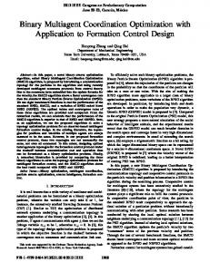
Figure 1: Flight paths that results after the coordination. Original flight paths were straight lines intersecting each other. Iterations from vehicles 1, 2 and 3

16

14

Value of local cost function

VEHICLE #1 ITERATIONS 12

VEHICLE #2 ITERATIONS 10

VEHICLE #3 ITERATIONS 8

6

4

0

2

4

6 Iteration

8

10

12

Figure 2: Value of local cost functions Fi (xi , βi |{xj }i ) during iterations on the solutions received for Scenario A.

decentralized optimization problem is the following: 11 We have introduced planar kinematics for simpler computational analysis. Refer to [Ghosh and Tomlin, 2000] for results which show that this kinematic model corresponds well to dynamics of the aircraft under nonlinear closed loop control.

Definition 9 (Implementation for which local constraints are always satisfied) A locally always feasible formulation of local optimization problem for ith subsystem for a given {xj }i , ∀j ∈ Ni is; min βi fi (xi ) + Pgi (xi |{xj }i )

xi ∈Sli

(31)

where the locally feasible set is defined as Sli = {xi : gli (xi ) ≤ 0, hli (xi ) = 0}

(32)

In our examples, hli and gli represent the planar dynamics and bounds on the velocity and turn rate of the ith vehicle. Based on the inherent decoupled structure of local dynamics, we propose an always local feasible implementation in which the subsystem dynamics and the input constraints are always satisfied while producing answers for the global coordination. The solutions generated by the vehicles correspond to trajectories over a finite time interval, T . We use the Matlab Optimization Toolbox function “fmincon” to solve this constrained problem and simulations are performed using the demo version of networking platform RBNB by Creare Inc. This setup allows multiple processes to run communicating through a common world model. In our simulations, communication links for the UAVs are modelled as binary erasure channels with capacities Cj = pj for the jth vehicle. Here pj corresponds to the probability that the message has been received by the ith vehicle. In our implementation, the local selection criterion at the kth step is max ∆Ftotal (k), which results in the maximum cost decrease. Also, we have fixed the penalty parameters for each vehicle to βi = βi (0) (based on the fact that they produced good results without local penalty parameter updates). The first example (Scenario A) is a general flight scenario, where the vehicles have to coordinate to satisfy the minimum separation constraint. Here, the imperfect communication channels are modelled as: p1 = 0.7, p2 = 0.8, p3 = 0.6, p4 = 0.9 for each aircraft. Figs. 1 and 2 show the flight paths and the convergence of the algorithm under communication losses after postprocessing. We have achieved the global coordination goals within a very tight tolerance (a few meters)12 . Lines of identical pattern, correspond to the value of Fi (xi , βi |{xj }i ) for each vehicle. Notice especially that a very bad link from vehicle 3 to 1 results in that solution not being updated for a long time as it is seen as a flat line on the local cost function plot of vehicle 1. When communication is restored, we obtain a better solution from vehicle 3. However, the graph indicates a solution of similar quality (cost) was indeed received beforehand. This illustrates the property of our algorithm in which solutions can flow down from different routes even though the communication between two vehicles is unreliable. The second example (Scenario B) is a perpendicular crossing (collision) pattern for four UAVs in a common airspace. The result of the coordination is shown in Fig. 3 in which all the safety constraints are satisfied within a few meters. 12 This ²-infeasibility can also be avoided by tightening the constraints until all of them are feasible.

6

Conclusions and Current Work

In this work, we have presented a decentralized optimization method for solving the coordination problem of interconnected nonlinear dynamic systems with multiple decision makers and incomplete mathematical models. The method covers a large class of problems where there is cooperation and solution passing in the system. In our current work, we have shown that second order sufficiency ˙ conditions [Inalhan et al., 2002] for Pareto-optimality of centralized problem can be guaranteed for cases in which there is dominating local convexity in the solution or when the interconnections are weak. The main conceptual barrier to general centralized Pareto-optimality comes from the fact that, even though common constraints are identical in interconnected systems, they are seen differently by each decision maker in the decentralized setting as they control only a subset of the global optimization variables.

References [Bertsekas and Tsitsiklis, 1997] Bertsekas, D. P. and Tsitsiklis, J. N. (1997). Parallel and Distributed Computation: Numerical Methods. Athena Scientific, Belmont, MA. [Cheng and Wellman, 1998] Cheng, J. Q. and Wellman, M. P. (1998). The WALRAS algorithm: A convergent distributed implementation of general equilibrium outcome. Computational Economics, 12(1):1–24. [de Miguel, 2001] de Miguel, A.-V. (2001). Two Decomposition Algorithms for Nonconvex Optimization Problems with Global Coordinated Safety Assurance

25 20 15 10

y [km]

5 0 −5 −10 −15 −20 −25 −25

−20

−15

−10

−5

0 x [km]

5

Figure 3: Scenario B

10

15

20

25

Coordinated Safety Assurance

20

15

10

5 y [km]

In addition, we have extended the technique we have developed to moving time horizons where each UAV ‘connects’ and ‘disconnects’ to the environment. Subsystem optimizations dynamically change in time as the vehicles come in communication proximity to each other. Fig. 4 presents all the solutions generated during decentralized optimization. Here each path corresponds to Tm seconds of flight solution proposed by a vehicle during the bargaining process. As time progress, the solution implemented is a piecewise combination of solutions found at each particular moving time horizon with end point penalties that approximate “cost-to-come”. Piecewise convergence of such a scheme is guaranteed at each step but total boundedness of the global cost is still an open issue.

0

−5

−10

−15

−20 −25

−20

−15

−10

−5

0 x [km]

5

10

15

20

25

Figure 4: Solutions generated during decentralized optimization via bargaining with moving time horizon, shown prior to any pruning. Variables. PhD thesis, Department of Management Science and Engineering, Stanford University, Stanford CA. [Frazzoli et al., 2001] Frazzoli, E., Mao, Z., Oh, J., and Feron, E. (2001). Aircraft conflict resolution via semi-definite programming. AIAA Journal of Guidance, Control, and Dynamics, 24(1):79–86. [Ghosh and Tomlin, 2000] Ghosh, R. and Tomlin, C. J. (2000). Nonlinear inverse dynamic control for mode-based flight. In Proceedings of AIAA/GNC Conference, Denver CO. [Heiskanen, 1999] Heiskanen, P. (1999). Decentralized method for computing pareto solutions in multi-party negotiations. European Journal of Operational Research, 117(3):578–590. [Hillermeier, 2001] Hillermeier, C. (2001). Nonlinear Multiobjective Optimization: A generalized homotopy approach. Birkhauser, Basel CH. [Hu et al., 2001] Hu, J., Prandini, M., Nilim, A., and Sastry, S. (2001). Optimal coordinated maneuvers for three dimensional aircraft conflict resolution. In Proceedings of AIAA/GNC Conference, Montreal PQ. ˙ ˙ [Inalhan et al., 2002] Inalhan, G., Stipanovi´ c, D. M., and Tomlin, C. J. (2002). Decentralized optimization, with application to multiple aircraft coordination. Technical Report SUDAAR - 759, Stanford University, Stanford CA. Submitted to JOTA. [Li and Ba¸sar, 1987] Li, S. and Ba¸sar, T. (1987). Distributed algorithms for the computation of noncooperative equilibria. Automatica, 23(4):523–533. [Luenberger, 1989] Luenberger, D. G. (1989). Linear and Nonlinear Programming. Addison Wesley, Reading, MA, second edition. [Luo et al., 1996] Luo, Z.-Q., Pang, J.-S., and Ralph, D. (1996). Mathematical Programs with Equilibrium Constraints. Cambridge University Press. [McLain et al., 2000] McLain, T. W., Chandler, P. R., and Pachter, M. (2000). A decomposition strategy for optimal coordination of unmanned air vehicles. In Proceedings of the American Control Conference, Chicago, IL. [Miettinen, 1999] Miettinen, K. M. (1999). Nonlinear Multiobjective Optimization. Kluwer Academic. ¨ uner and Perkins, 1978] Ozg¨ ¨ uner, U. and Perkins, W. R. [Ozg¨ (1978). Optimal control of multilevel large-scale systems. International Journal of Control, 28(6):967–980. [Verkama et al., 1994] Verkama, M., Ehtamo, E., and Hamalainen, R. P. (1994). On distributed computation of Pareto solutions in n-player games. Research Report A53, Helsinki University of Technology, Systems Analysis Laboratory. ˇ ˇ [Siljak, 1991] Siljak, D. D. (1991). Decentralized Control of Complex Systems. Academic Press, New York, NY.