Optimization Problems in Multiple-Interval Graphs - CiteSeerX

Optimization Problems in Multiple-Interval Graphs Ayelet Butman1 , Danny Hermelin?2 , Moshe Lewenstein3 , and Dror Rawitz4 1

Department of Computer Science, Holon Institute of Technology, Holon - Israel. [email protected] 2 Department of Computer Science, University of Haifa, Mount Carmel, Haifa 31905 - Israel. [email protected] 3 Department of Computer Science, Bar Ilan University, Ramat Gan 52900, Israel. [email protected] 4 Caesarea Rothschild Institute, University of Haifa, Mount Carmel, Haifa 31905 - Israel. [email protected]

Abstract. Multiple-interval graphs are a natural generalization of interval graphs where each vertex may have more then one interval associated with it. We initiate the study of optimization problems in multipleinterval graphs by considering three classical problems: Minimum Vertex Cover, Minimum Dominating Set, and Maximum Clique. We describe applications for each one of these problems, and then proceed to discuss approximation algorithms for them. Our results can be summarized as follows: Let t be the number of intervals associated with each vertex in a given multiple-interval graph. For Minimum Vertex Cover, we give a (2 − 1/t)approximation algorithm which equals the best known ratio for 2t − 1 bounded degree graphs. Since these graphs are known to be included in multiple-interval graphs with t intervals associated to each vertex, this ratio is in some sense tight. Following this, we give a t2 -approximation algorithm for Minimum Dominating Set which adapts well to more general and restricted variants of the problem. We then proceed to prove that Maximum Clique is NP-complete for the case of t = 3, and provide a (t2 − t + 1)/2approximation algorithm for the problem, using recent bounds proven for the so-called transversal number of t-interval families.

and storage problems translate to finding minimum colorings and clique covers in appropriate interval graphs [18]. A natural generalization of interval graphs are multiple-interval graphs. A multiple-interval graph is an intersection graph of a family of multiple intervals, where a multiple-interval is the union of a finite number of disjoint intervals over the real line. Many problems that translate to interval graph problems extend naturally to multiple-interval graph problems. Scheduled tasks become multi-tasks, storage items require non-linear storage space, and so forth. However, in contrast to interval graphs, most of these problems turn out to be NP-hard. In this paper, we consider three classical optimization problems in multiple-interval graphs: Minimum Vertex Cover, Minimum Dominating Set, and Maximum Clique. Since all three are NP-hard, our study focuses on designing approximation algorithms for these problems. 1.1

Applications and motivation

Interval graphs and closely related relatives have been studied extensively due to their wide applicability for modeling many real life problems. Below, we consider three applications that correspond to the three problems we consider for multiple-interval graphs in this paper.

Loss Minimization: Maximum Independent Set is probably the most widely applicable problem in multiple-interval graphs [8, 9]. Usually, the applicaInterval graphs are one of the most popular and well- tions for this problem are in scheduling or resource alunderstood graph classes in algorithmic graph theory. location scenarios. Since Minimum Vertex Cover They have numerous applications in various areas, is the complement problem of Maximum Indepenmost of which can be modeled by classical graph- dent Set, once can apply this problem in most of theoretic problems. As an example, basic scheduling these scenarios, where one is interested in minimizing ? Partially supported by the Israel Science Foundation loss occurring due to unscheduled tasks or unfulfilled grant 282/01. allocation requests.

1

Introduction

2

For instance, [8] describes an application for Minimum Independent Set in transmission of continuous-media data such as video by demand. Here, each multiple-interval represents multiple time segments in which a client requests data, allowing him to see a movie for instance, with intermediate breaks. Two client requests are in conflict if there is some time period in which they overlap. An optimal schedule therefore corresponds to the maximum (weight) independent set in the corresponding multiple-interval graph. In terms of loss minimization, the minimum loss is obtained by not supplying the requests which correspond to the minimum weight vertex cover in the corresponding multiple-interval graph. Another application mentioned in [8] is scheduling RAM and processor time for multiple real-time programs on multi-tasking systems. Here, loss minimization corresponds to the minimum number of programs to be removed from the schedule so that all remaining programs can run concurrently. We mention also that loss minimization for 1-interval requests, where intervals have an additional demand attribute associated with them, has been considered by Bar-Noy et al. [5]. Employee Monitoring: Consider the following scenario: The sales manager of the ACME department store chain wants to monitor the salespersons at one of his stores, since sales are not looking too good this year. For this, he ensembles a group of monitor employees from the entire ACME chain, who’s job is to inspect the salespersons of the store during their work shift. Now, at the beginning of each week he is handed the working schedule of all the salespersons in the store, in addition to the working schedule of the monitoring employees. Each schedule is represented by a multiple-interval which corresponds to multiple shifts in the week, i.e. multiple time segments in which the salesperson or monitor can be at the store. The manager seeks to find the minimum number of monitor employees needed to inspect each one of salespersons at least once during the week, so the remaining monitor employees can be assigned monitor duties in other stores of the ACME chain. If we assume that for a salesperson to be inspected by a monitor, it is enough that they are both together in the store for some time period during the week, the problem above translates to Minimum Dominating Set where the multiple-intervals corresponding to salespersons are assigned infinite weight. Communication Clique: Suppose you want to organize an international workshop of computer science

specialists. In your community, you have many people fluent in many different languages. You wish to invite as many specialist as possible, but you want all them to be able to communicate together since you’re on a tight schedule and anxious to obtain the long anticipated breakthrough in your research. If we consider the real line as a discrete set of finite points, where each point represents a different langauge, we can assign a multiple-interval (where each interval is a single point) to each specialist in the community, according to the multiple languages he is fluent in. The problem above then translates to Maximum Clique in the corresponding multiple-interval graph. One can imagine that the scenario described above appears in other real-life situations, e.g. servers and communication protocols, transmitters and frequency intervals, and so forth. 1.2

Our results

We initiate the study of combinatorial optimization problems on multiple-interval graphs. As mentioned above, our study focuses on three classical problems: Minimum Vertex Cover, Minimum Dominating Set, and Maximum Clique. Below, we briefly describe our results for each of these problems. We use the term t-interval to refer to a multiple-interval which is the union of t disjoint intervals. For Minimum Vertex Cover, we give a (2 − 1/t)-approximation algorithm, which equals the current best known ratio for 2t − 1 bounded degree graphs [25]. Since t-interval graphs include 2t − 1 bounded degree graphs [20], this, in some sense, is the best that we can hope for. Our algorithm consists of two phases. The first phase is a clean-up phase that is based on the local ratio technique. At the end of this phase, the remaining t-interval graph is hereditarily sparse, i.e. each of its induced subgraphs is sparse. In the second phase we apply known techniques for computing vertex covers in hereditarily sparse graphs. For Minimum Dominating Set, we present a t2 approximation algorithm which also applies for the more general case in which we are given two subsets: a subset B ⊆ F that contains t-intervals that should be dominated, and a subset R ⊆ F that contains t-intervals that may be used to dominate the t-intervals in B. This more general version of the problem is equivalent to Minimum Directed Dominating Set, since we do not require R and B to be disjoint. Our algorithm can also be applied when B contains tB -intervals and R contains tR -intervals, and in this case it computes (tB · tR )-approximate solutions. We note that this version of the problem contains problems such as Minimum Rectangle

3

Transversal (tB = 2, tR = 1, and the intervals in R are points), Minimum t-Interval Transversal (tB = t, tR = 1 and the intervals in R are points), and Minimum Set Cover with at most t blocks of consecutive ones in each column of the constraint matrix (tB = 1, tR = t, and the intervals in B are points) as special cases. In fact, our algorithm extends the 2-approximation algorithm for Minimum Rectangle Transversal from [17], the t-approximation algorithm for Minimum t-Interval Transversal that is implied by combining [23, 24], and the t-approximation algorithm for Minimum Set Cover with at most t blocks of consecutive ones from [26]. Maximum Clique differs from the two problems above in that it was previously unknown whether the problem was hard, even for large values of t. We prove that Maximum Clique is already NP-complete for the case of t = 3. In addition, we present a (t2 − t + 1)/2-approximation algorithm for the problem, using recent bounds proven for the transversal number of t-interval families in [28]. 1.3

Related work

Multiple-interval graphs have been studied extensively from the graph-theoretic aspect. We briefly list some of the main results. The class of graphs with maximum degree ∆ are d(∆ + 1)/2e-interval graphs [20], while the complete bipartite graph Km,n is a d(mn + 1)/(m + n)e-interval graph. Every graph with n vertices is a d(n+1)/4e-interval graph, and the complete bipartite graph Kbn/2c,dn/2e is an extremal example of this [19]. The class of planar graphs is a subclass of 3-interval graphs [33]. Finally, the problem of determining whether a given graph is t-interval is NP-complete for t ≥ 2 [36]. Many variants of multiple-interval covering problems have been studied by the combinatorial optimization and discrete geometry communities. Hochbaum and Levin [26] studied the problem of covering points by t-intervals. The inverse problem of covering t-intervals by points, also called Minimum t-Interval Transversal, has been studied along with many of its variants in [17, 22–24]. Obtaining upper bounds for the transversal number of any tinterval family has been considered by [2, 21, 28, 34]. Computational biology is another field where multiple-interval graph problems have been recently considered. For instance, Bafna et al. [4] studied the problem of finding the maximum weight subset of non-overlapping local alignments between two genomic sequences. This problem translates to finding a

maximum weight independent set in a restricted subclass of 2-interval graphs. In [3], the authors studied another restricted subclass of t-interval graphs in the context of high throughput genotyping. In [11, 15, 35], 2-intervals were used to model secondary structure of RNA sequences, and secondary structure prediction scenarios were modeled by variants of the Maximum Independent Set problem in 2-interval graphs. Classical optimization problems have been considered on several ”geometric” intersection graphs. The first results of these type are now part of the classic literature [12, 18, 31]. Recently, this line of research has been extended to consider intersection graphs of various types of geometric objects, e.g. intersection graphs of discs or ellipses in the plane [14, 16, 27], intersection graphs of axis parallel rectangles [1, 10], and intersection graphs of general fat objects [13]. Finally, probably the most relevant work to ours is that of Bar-Yehuda et al. [8] who studied the Maximum Independent Set problem in t-interval graphs. They gave a 2t-approximation algorithm for this problem, in addition to a 2t-approximation algorithm for the Minimum Coloring problem. We mention also [9], where a more general variant of Maximum Independent Set has been studied. 1.4

Basic notations and terminology

We next briefly discuss notation and terminology that will be used throughout the paper. Let i1 , i2 , . . . , it be t disjoint closed intervals of the real line. The t-interval I = (iS 1 , i2 , . . . , it ) is the union t of these t intervals, i.e. I = j=1 ij . Given a pair of t-intervals I = (i1 , i2 , . . . , it ) and J = (j1 , j2 , . . . , jt ), these two t-intervals intersect if they share a common St St point, i.e. ( k=1 ik ) ∩ ( `=1 j` ) 6= ∅. Let F = {I1 , . . . , In } be a family of t-intervals. The underlying family of intervals of F, denoted I(F), is the family of all intervals that compose © the t-intervals¯ in F. That is, I(F) i ∈ ª = {i1 , i2 , . . . , it } ¯ I = (i1 , i2 , . . . , it ) ∈ F . The intersection graph ΩF of F, is a graph with a one-to-one correspondence between its vertices and F such that two vertices are connected in ΩF if their corresponding t-intervals in F intersect. We say that ΩF is a t-interval graph to emphasis that it is an intersection graph of family of t-intervals for some given t ∈ N+ . We are concerned with vertex covers, dominating sets, and cliques in t-interval graphs. In terms of tinterval families, a subset C ⊆ F is a cover of F if F \ C is pairwise disjoint. A subset D of a t-interval family F is a dominating set of F if for any t-interval in F \ D there is a t-interval in D which intersects

4

it. A subset K ⊆ F is called a clique if it is pairwise intersecting. Given a weight function w : F → Q+ , the Minimum Vertex Cover and Minimum Dominating Set problems in t-interval graphs ask to find the minimum weight cover and dominating set of F, and the Maximum Clique problem asks to find the maximum weight clique of F. A subset C ⊆ F is an α-approximate cover of F, if C is a cover of F with w(C) ≤ α · w(Copt ), where Copt is the minimum cover of F. We define α-approximate dominating sets and cliques of F similarly.

for F such that w = w1 +w2 . Then, if C ⊆ F is an αapproximate cover for F, both with respect to w1 and with respect to w2 , then C is also an α-approximate cover with respect to w.

A typical local ratio algorithm is recursive. In each recursive step, the algorithm first collects all zero elements to its solution. It then defines a weight function w1 in such a way that w2 = w − w1 still assigns nonnegative weights to all elements, and at least one element with non-zero weight with respect to w will get zero weight with respect to w2 . The algorithm then recursively solves the instance of the problem with w2 2 Minimum Vertex Cover as the given weight function, and fixes the returned solution so it will be a good approximate solution In the following section we consider the Minimum with respect to both w1 and w2 . By the Local-Ratio Vertex Cover problem for t-interval graphs. Re- theorem, this solution is guaranteed to be a good apcall that 2t − 1 bounded degree graphs are t-interval proximation with respect to w as well. graphs [20], and so Minimum Vertex Set is APXIn Figure 1 we present algorithm LR-Cover which hard in t-interval graphs with t ≥ 2, by the APX- applies the Local-Ratio technique for cleaning F. A hardness results given in [32] for bounded degree similar cleaning phase was used in [7] in order to get graphs. We present an approximation algorithm with rid of short odd cycles in the input graph. In its reperformance ratio 2 − 1/t for the problem, which cursive basis, algorithm LR-Cover invokes algorithm equals the best known approximation ratio for Min- Flat-Cover which specializes in flat t-interval families. imum Vertex Cover in 2t − 1 bounded degree We may assume with out loss of generality that the graphs [25]. initial weight function w is positive. The general outline of our algorithm is as follows. We first initiate a cleaning phase on F. At the end of this phase, we remain with a family of t-intervals Algorithm LR-Cover(F , w) F 0 ⊆ F which has the following convenient propData : A set of t-intervals F and a weight erty: There are no three pairwise intersecting interfunction w : F → Q+ . 0 vals in the underlying interval family of F , or in Result : A cover C of F . begin other words, ΩI(F 0 ) does not contain a clique of size 1. if F is flat then return Flat-Cover(F, w). three. We call t-interval families with this property 2. Select an endpoint p with |Kp | ≥ 3, where flat. Flat t-interval families are convenient for our Kp = {I ∈ F | p ∈ I}. purposes since their intersection graphs are heredi3. Select I0 ∈ Kp with ( w(I0 ) = minI∈Kp w(I). tarily sparse (every induced subgraph is sparse), and w(I0 ) I ∈ Kp , we can apply known techniques for these types of 4. Define w1 (I) = . 0 otherwise graphs. The crux is therefore in the cleaning phase. 5. Define w2 = w − w1 . We show that we can clean F in order to obtain a 6. F + ← {I ∈ F | w2 (I) > 0}. 0 0 0 flat subset F ⊆ F in such a way that if C ⊆ F is 7. C ← LR-Cover(F +, w2 ). an α-approximate cover of F then C 0 ∪ (F \ F 0 ) is 8. C ← C ∪ {I ∈ F | w2 (I) = 0}. a max{α, 1.5}-approximate cover of F. Hence, using return C. the known algorithm for hereditarily sparse graphs, end we obtain our desired 2 − 1/t ratio. Fig. 1. Algorithm LR-Cover.

2.1

The cleaning phase

The cleaning phase is based on the Local-Ratio techLemma 1. Suppose that algorithm Flat-Cover is an nique [7] which in turn is based on the Local-Ratio α-approximation algorithm for the Minimum VerTheorem. In our terms, this theorem is stated as foltex Cover problem in flat t-interval graphs. Then lows. algorithm LR-Cover is a max{α, 1.5}-approximation Theorem 1 (Local Ratio [7]). Let F be a family of algorithm for Minimum Vertex Cover in general t-intervals and let w, w1 , and w2 be weight functions t-interval graphs.

5

Proof. First observe that at each recursive call of LRCover, the size of F decreases at least by one, since the t-interval I0 selected at step 4 is excluded (along with possibly other t-intervals) from the next recursive call. Hence, LR-Cover invokes Flat-Cover after ` ≤ n recursive calls, and is guaranteed to terminate assuming Flat-Cover terminates as well. The proof is by induction on the recursive calls of LR-Cover. At the `’th recursive call, the lemma follows by the assumption that Flat-Cover is an α-approximation algorithm for flat families of t-intervals. Consider therefore, the i’th recursive call of LR-Cover, i ≤ `, and assume the lemma follows for any j’th call, i < j ≤ `. Let (F, w) be the instance at the ith recursive call, and let C ⊂ F be the family of t-intervals computed at step 7. Set β = max{α, 1.5}. By the inductive hypothesis, C is a β-approximate cover for F + with respect to w2 . Step 8 ensures that C is also a cover for F, since all t-intervals in F \ F + are added to C. Also, after step 8, C remains β-approximate with respect to w2 , since only t-intervals with zero w2 -weight have been added to C at this step. We argue that after step 8, C is also β-approximate with respect to w1 . Let optw1 be the weight of the optimal cover of F with respect to w1 , and let Kp be the subset of t-intervals defined at step 2. Set ε to be the weight of the t-interval I0 selected at step 3. Since Kp is pairwise intersecting, any cover for F must include at least |Kp | − 1 t-intervals of Kp . Hence, since w(I) = ε for any I ∈ KP p , we have ε(|Kp |−1) ≤ optw1 . On the other hand, I∈F w1 (I) = ε|Kp |, and so P I∈C w1 (I) ≤ ε|Kp |. It then follows that P ε|Kp | 3 I∈C w1 (I) ≤ ≤ ≤ β, optw1 ε(|Kp | − 1) 2 where the second inequality follows from the fact that |Kp | ≥ 3. We have shown that at any recursive call of LRCover, the cover C returned is β-approximate both with respect to w1 and w2 . Applying the Local-Ratio Theorem, we obtain that C is β-approximate with respect w at any recursive call, and we are done. t u 2.2

Flat t-interval families

A graph is hereditarily sparse, if each one of its induced subgraphs has a bounded average degree. The following lemma proves that the intersection graph of any flat t-interval family is hereditarily sparse. Lemma 2. Let F be a flat t-interval family, |F| = n, and let G = ΩF be the intersection graph of F. Then |E(G)| ≤ tn − 1.

Proof. Consider the interval graph G∗ = ΩI(F) , the intersection graph of the underlying set of intervals of F. Since any edge of G corresponds to at least one edge of G∗ , we have |E(G)| ≤ |E(G∗ )|. Furthermore, since any vertex in G corresponds to at most t vertices of G∗ , we have |V (G∗ )| ≤ t|V (G)|. To complete the proof, we argue that |E(G∗ )| ≤ |V (G∗ )| − 1 by showing that G∗ does not contain any cycles. To see this, note that G∗ is an interval graph, and as such it is also chordal [18]. Hence, if it contains a cycle, it also contains a clique of size three, contradicting the fact that F is flat. Combining all inequalities together, we get |E(G)| ≤ |E(G∗ )| ≤ |V (G∗ )|−1 ≤ t|V (G)|−1 = tn−1, and the lemma follows.

u t

In [25], Hochbaum presented a (2 − 2/k)approximation algorithm for Minimum Vertex Cover in graphs that can be colored in k colors. When F is flat, Lemma 2 implies that ΩF can be colored by 2t colors, and therefore, in this case we can find an (2 − 1/t)-approximate cover for F using Hochbaum’s algorithm. Lemma 3. If F is a flat t-interval family then one can find a (2 − 1/t)-approximate cover for F in polynomial time. By invoking Lemma 1 with the algorithm promised by Lemma 3 as algorithm Flat-Cover, we obtain the main result of this section. Theorem 2. The Minimum Vertex Cover problem in t-interval graphs can be approximated in polynomial time within a factor of 2 − 1/t.

3

Minimum Dominating Set

In the following section we study the Minimum Dominating Set problem for t-interval graphs. The problem is APX-hard for t ≥ 2 via [20] and [32]. For the case of t = 1 (interval graphs), we present an algorithm based on the primal-dual method [6] which computes optimal solutions. Afterwards, we present a t2 -approximation algorithm for the case of t-interval graphs using a reduction to interval graphs. For ease of presentation, we will solve a slightly more general variant of Minimum Dominating Set in which we are given two families of t-intervals, the red family R = {I1 , . . . , In } and the blue family B = {J1 , . . . , Jm }, and the requirement is to find a minimum weight subset of R which dominates B. We

6

do not require the two families to be disjoint, and so if R = B our variant reduces to the original Minimum Dominating Set problem. Naturally, we assume that for every blue t-interval in B there is at least one red t-interval in R which dominates it. 3.1

Linear programming formulation

We next briefly describe linear programming terminology that is essential for describing our algorithm. We assume basic knowledge of linear programming. Readers unfamiliar with the subject are referred to [29]. Let x(I) denote a real variable associated with the red t-interval I ∈ R. Our generalized variant of minimum Dominating Set can be formalized using the following linear integer program. P min PI∈R w(I)x(I) s.t. (DS) I : J∩I6=∅ x(I) ≥ 1 ∀J ∈ B x(I) ∈ {0, 1} ∀I ∈ R where x(I) = 1 if I is in the dominating set. The linear relaxation of DS is obtained by replacing the integrality constraints by: x(I) ≥ 0, for every I ∈ R. We denote the linear relaxation of DS by LP-DS. The integrality gap of DS is the ratio between the optimal solutions of DS and LP-DS. The dual program of LP-DS is: P max PJ∈B y(J) s.t. J : I∩J6=∅ y(J) ≤ w(I) ∀I ∈ R y(J) ≥ 0 ∀J ∈ B Here, the variables y(J) correspond to blue t-intervals J ∈ B. LP-DS is regarded as the primal program with respect to its dual. We will use x and y to denote primal and dual solution vectors respectively. A primal or dual solution is said to be feasible if it is indeed subject to all its corresponding constrains. It is known that for any pair soluP P of feasible primal-dual tions x and y we have I∈R w(I)x(I) ≥ J∈B y(J), and are both optimal if and only if P that x and yP J∈B y(J). I∈R w(I)x(I) = We will the need the so-called complementary slackness conditions. For LP-DS, these conditions are stated as follows:

3.2

Algorithm for interval graphs

We next present a primal-dual algorithm that computes optimal dominating sets for 1-interval graphs. Our algorithm starts with a pair of primal-dual solutions x = 0 and y = 0. It has two phases. In the first, it gradually converts the primal solution to a feasible solution, while maintaining its integrality and the feasibility of the dual solution. The second phase is a reverse deletion phase, where the algorithm converts the primal solution to an optimal one, by assuring that the complementary slackness conditions are met. Figure 2 depicts our primal dual algorithm PDDominate. We assume that x = 0 and y = 0 are the initial primal-dual solution vectors. Furthermore, we assume that the blue intervals B = J1 , . . . , Jn are ordered in non-decreasing order of right endpoints. Algorithm PD-Dominate(R, B, w) Data : Two families of intervals R = {I1 , . . . , In } and B = {J1 , . . . , Im }, and a weight function w : R → Q+ . Result : A dominating set D ⊆ R of B. begin 1. for ` = 1 . . . m do if J` does not intersect an interval I ∈ R with x(I) = 1 then (a) Increase y(J` ) until some dual constraint becomes tight. (b) Select a red interval I ∈ R corresponding to a dual constraint that has just become tight. (c) Set x(I) = 1. end end 2. for ` = m . . . 1 do if y(J` ) > 0 then (a) Let x(I) be the variable which was set to 1 due to J` . (b) If the primal solution remains feasible when x(I) is set to zero then set x(I) = 0. end end return D = {I ∈ R | x(I) = 1}. end Fig. 2. Algorithm PD-Dominate

– P The primal conditions: ∀I ∈ R : x(I) ≥ 0 ⇒ J : I∩J6=∅ y(J) = w(I). Lemma 4. Algorithm PD-Dominate computes an – The P dual conditions: ∀J ∈ B : y(J) ≥ 0 ⇒ optimal dominating set D ⊆ R of B. x(I) = 1. I : J∩I6=∅ A pair of feasible primal-dual solutions x and y are both optimal if and only if they both satisfy the complementary slackness conditions.

Proof. The pair of primal and dual solutions x and y are both feasible by construction. To prove the lemma, we show that x is optimal by showing that

7

both x and y satisfy the complementary slackness conditions. First, by the construction of the primal solution, a primal variable is set to 1 only if its corresponding dual constraint is tight. Hence, the primal conditions are satisfied. To finish the proof we need to show that the dual conditions P are also satisfied, namely, that if y(J) > 0 then I : J∩I6=∅ x(I) = 1, for every J ∈ R. Equivalently, we show that after the reverse deletion phase, if y(J) > 0, then there is exactly one red interval I that dominates J with x(I) = 1. We prove this claim using induction on the blue intervals in reverse order (Jn , . . . , J1 ). At the recursive base, there are no intervals and there is nothing to prove. For the inductive step, we assume that the intervals J`+1 , . . . , Jn satisfy the claim, and show that it holds for J` as well. If y(J` ) = 0, then we are done. Otherwise, if y(J` ) > 0, it follows that when the algorithm reached J` in the first phase, x(I) = 0 for every red interval I ∈ R that intersects J. Hence, J` can only be dominated in D by red intervals that were taken after reaching J` in the first phase. If J` is the rightmost interval with non-zero dual variable we are done. Otherwise, let Jk be the closest interval to the right of J` with non-zero dual variable. By the inducP tive assumption we know that I : Jk ∩I6=∅ x(I) = 1. Hence, when the algorithm returns to J` in the reP verse deletion phase I : J` ∩I6=∅ x(I) ≤ 2. Since the algorithm removes the red interval whose primal variable was set to 1 duePto J` in case feasibility is maint u tained, we get that I : J` ∩I6=∅ x(I) = 1. The following is implied by the optimality of the primal-dual pair and the integrality of the primal solution. Corollary 1. The integrality gap of DS is 1 in the case of t = 1. 3.3

Algorithm for t-interval graphs

We are now in position to present our t2 approximation algorithm for t-interval families. Our algorithm starts by solving the linear program LPDS. Following this, it uses the optimal solution of LP-DS to construct an instance for the case of t = 1. A t2 -approximate solution for the original instance is then constructed from the optimal solution of the new instance. Let x∗ denote an optimal solution of LP-DS. We assume without loss of generality that each red t-interval in R consists of unique t intervals, i.e. that |I(R)| = t|R|. For a given blue t-interval J = (j1 , . . . , jt ) ∈ B, we select a unique representative

P j ∈ {j1 , . . . , jt } which maximizes I∈R,I∩j6=∅ x∗ (I). In other words, the representative j is the maximum dominated interval of J. We construct a new 1-interval instance (R0 , B 0 , w0 ) as follows: – R0 = {I 0 = i | i ∈ I(R)}. – B0 = {J 0 = j | J ∈ B, j represents J}. – w0 (I 0 ) = w(I)/t, where I 0 = i, i ∈ I(R), and I is the unique red t-interval which consists of i. We now invoke PD-Dominate(R0 , B0 , w0 ). Let D ⊆ R0 be the dominating set returned by PDDominate(R0 , B0 , w0 ). We return the solution D = 0 0 {I of I}. Note that P ∈ R | I ∈ PD is an0 interval 0 w(I) ≤ t · w (I ), and that this inequal0 I∈D I ∈D ity is tight in case no two intervals of a t-interval in D are together in D0 . 0

Lemma 5. D is a t2 -approximate dominating set of B. Proof. First note that by the construction of the algorithm above, D is a dominating set of B. Let x and x0 be the solution vectors corresponding to D and 0 D we show that P the lemma, P, respectively. To2 prove ∗ w(I)x (I). w(I)x(I) ≤ t · I∈R I∈R We define a fractional solution x ¯ for the instance (R0 , B0 , w0 ) as follows: x ¯(I 0 ) = t · x∗ (I), where I 0 = i, i ∈ I(R), and I is the unique red t-interval which consists of i. Notice that X X w0 (I 0 )¯ x(I 0 ) = t · w(I)/t · (t · x∗ (I)) I 0 ∈R0

I∈R

=t·

X

w(I)x∗ (I).

I∈R

We argue that x0 is feasible with respect to (R0 , B0 , w0 ). To see this, consider any blue t-interval J = (j1 , ..., jt ) and its representative J 0 ∈ {j1 , ..., jt }. By P our selection of J 0 , I∈R,I∩J 0 6=∅ x∗ (I) ≥ 1/t, since otherwise P x∗ would not be feasible. From this it fol¯(I 0 ) ≥ 1 for any J 0 ∈ R0 . lows that I 0 ∈R0 ,I 0 ∩J 0 6=∅ x We know that x0 is an optimal solution for (R0 , B0 , w0 ). Hence, the weight of x ¯ is at least as high as the weight of x0 . Furthermore, by Corollary 1, we can assume that x0 is integral. It follows that X X w(I)x(I) ≤ t · w0 (I 0 )x0 (I 0 ) ≤ I 0 ∈R0

I∈R

t·

X

w0 (I 0 )¯ x(I 0 ) = t2 ·

I 0 ∈R0

and we are done.

X

w(I) · x∗ (I),

I∈R

u t

The following theorem summarizes the main result of this section.

8

Theorem 3. The Minimum Dominating Set problem in t-interval graphs can be approximated in polynomial time within a factor of t2 .

may choose any interval as a representative. We assume that for a given i ∈ {1, . . . , t + 1}, the algorithm chooses representatives in different segments for each t-interval Ii,j , j ∈ {1, . . . , t}. Hence, the 1-interval instance that is constructed by the algorithm contains 3.4 Tightness of analysis two blue intervals in each segment Si,i0 . Since all segments are disjoint, it follows that any We next show that the analysis of our algorithm is essentially tight. Specifically, we show that for every solution of the 1-interval instance must contain at 0 t ≥ 2, there exists an instance on which ¡ the ¢ algorithm least one red interval in each segment Si,i . Since there can be any order between the red intervals in each computes a solution whose weight is t+1 , while the ¡ ¢ 2 segment, a solution that contains t+1 red intervals, optimum is 1. 2 We describe an instance that consists of a family each belonging to a different t-interval, is feasible and F of t(t + 1) t-intervals. First, we define a family of t- optimal. In this case,¡ the ¢ solution returned by the t+1 t-intervals, and therefore intervals F¡ 0 =¢{I1 , . . . , It+1 }, by partitioning the real algorithms contains 2 ¡t+1¢ line into t+1 segments, and then placing in each its weight is as required. 2 2 segment Si,i0 , {i, i0 } ⊆ {1, . . . , t + 1}, two identical intervals, one belonging to Ii , and the other belonging to Ii0 . Then, we define F as the family which consists 4 Maximum Clique of t identical copies of each t-interval F 0 , where Ii,j ∈ F is the j’th copy of Ii ∈ F 0 . An example of this In the following section we consider the Maximum Clique problem. We show that the problem is hard construction with t = 3 is given in Figure 3. for t-interval graphs with t ≥ 3. Following this, we give a simple approximation algorithm for the problem which relies on recent bounds obtained for the I1,j transversal number of t-interval families (see Definition in Section 4.2). I 2,j

I3,j

4.1 j = 1, j = 2, j = 3.

I4,j S1,2

S1,3

S1,4

S2,3

S2,4

S3,4

Fig. 3. The t-interval family F for t = 3.

We now make two observations. First, note that the family of t-intervals F is pairwise intersecting, i.e. it is a clique. Second, note that we can determine any order between the intervals in each segment while making sure that F remains pairwise intersecting. Now, since F is a clique it follows that any tinterval in F constitutes a dominating set. Assuming unit weights, any t-interval is also an optimal solution. We show that in the case of unit weights the algorithm may compute a solution whose weight is ¡t+1¢ . 2 We assume that the algorithm starts with the fractional optimal solution x∗ , where x∗ (Iij ) = 1/t(t + 1). Observe that x∗ is indeed optimal. Now, in this case, each t-interval is equally dominated in each of its intervals. It follows that the algorithm

NP-hardness result

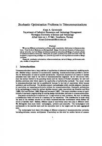
We begin by showing that Maximum Clique is NPhard in 3-interval graphs. We show this be presenting a reduction from Maximum 2-DNF. Recall that in Maximum 2-DNF, we are asked to determine whether one can satisfy at least k clauses in a given 2-DNF formula. That is, whether there is a truth assignment to the boolean variables of the formula, such that the value of at least k clauses in the formula is TRUE under this assignment. Maximum 2DNF is NP-hard due to the hardness result given in [30] for Minimum 2-CNF. We initially show that the weighted variant of Maximum Clique is NPhard, and then relax the weighted condition. Let Φ = D1 ∨ · · · ∨ Dm be a 2-DNF formula over a set of variables {x1 , · · · , xn }. We construct a 3interval family F which contains a 3-interval for each clause and each literal (i.e. variable with or without negation). For convenience, we will describe our construction by defining the underlying interval family IF of F over three disjoint segments I, II, and III, of the real line. In segment I, we first place 2n disjoint intervals, one for each literal 3-interval in F. Then, we define a 3-interval in F corresponding to each clause Di ∈ Φ as follows: Suppose Di consists of the two literals α

9

and β. The 3-interval of Di is the 3-interval obtained by taking an interval which covers all of segment I, and then removing from it the two intervals that correspond to the negations of α and β. In this way, all 3-intervals that correspond to clauses are pairwise intersecting, since all of them contain, for instance, the right boundary point of segment I. Figure 4 gives an example of our construction at this segment.

x1

x1

x2

x2

x3

x3

x4

x4

D1 D2 D3 D4 Fig. 4. An example of the construction at segment I. The clauses in this example are D1 = (¯ x1 ∧ x ¯2 ), D2 = (x2 ∧x3 ), D3 = (x1 ∧ x4 ), and D4 = (¯ x3 ∧ x ¯4 ).

literals and those corresponding to negative literals is reversed. Lemma 6. Let I ∈ F be a 3-interval corresponding to a literal α. Then I intersects all other 3-intervals in F which correspond to literals, except the 3-interval which corresponds to the negation of α. Proof. Assume w.l.o.g. that α is some positive literal xi . Then by construction, the 3-interval which corresponds to x ¯i does not intersect I. Furthermore, all 3-intervals which correspond to the other positive variables intersect I in segment II. To complete proof note that for all j < i, the 3-interval which corresponds to literal x ¯j intersects I in segment II, and for all j > i, the 3-interval which corresponds to literal x ¯j intersects I in segment III. u t We now assign to each 3-interval which corresponds to a literal weight m + 1 (= the number of clauses + 1), and to each 3-interval corresponding to a clause weight 1. We claim that this yields the following:

Lemma 7. There is a clique K ⊆ F of weight (m + 1)n + k iff there is an assignment that satisIn segment II, we first place n disjoint intervals, fies k clauses of the 2-DNF formula Φ. one for each 3-interval in F which corresponds to a Proof. Assume that there is an assignment satisfypositive literal. The intervals are placed in the or- ing k clauses of Φ. Let KX ⊆ F be the subset der of the variables, i.e. the interval corresponding of 3-intervals corresponding to this assignment, and to xi is placed to the left of the interval which cor- KD ⊆ F be the 3-intervals which correspond to the k responds to xi+1 . Next, for all 1 ≤ i < n, we add satisfied clauses of Φ. Then KX is pairwise intersectan interval corresponding to x¯i that begins at the ing by Lemma 6, and KD is pairwise intersecting by left endpoint of the interval corresponding to xi+1 construction. Furthermore, each I ∈ KX intersects and ends at the right boundary point of segment II. each J ∈ KX in segment I, since the assignment corThe interval which corresponds to x ¯n is placed to the responding to KX satisfies all clauses with 3-intervals right of the interval corresponding to xn . In this way, in KD . It follows that K = KX ∪ KD is a clique in F, all intervals corresponding to negative literals in this with weight (m + 1)n + k as desired. segment, intersect at at the right boundary point. Conversely, assume that there is an (m + 1)n + k weighted clique. Since the overall number of clauses is m it must be that the clique is formed from 3-intervals x1 x2 x3 x4 of n literals and k clauses. Since, by Lemma 6, xi and x¯i cannot be in a clique, the n variables form x1 an assignment. By construction, as observed above, each clause corresponding to a t-interval in the clique x2 must be satisfied. u t x3 x4

Fig. 5. Segment II.

This immediately implies that the weighted variant of Maximum Clique is NP-hard in 3-interval graphs. This line of proof can be extended to show that the same is true for the unweighted variant by constructing m + 1 identical copies of each 3-interval corresponding to a literal, instead of one 3-interval of weight m + 1.

Segment III is defined symmetrically to II, where Theorem 4. Maximum Clique is NP-hard in tthe roles of the intervals corresponding to positive interval graphs for t ≥ 3.

10

4.2

Approximation algorithm

We next present a (t2 − t + 1)/2 approximation algorithm for Maximum Clique. We begin with defining the notion of a transversal of a t-interval family: A transversal of F is a set of points {p1 , p2 , . . . , pτ } such that for every I ∈ F there is at least one pi ∈ {p1 , p2 , . . . , pτ } with pi ∈ I. The transversal number of F, denoted τ (F), is the minimum size of any transversal of F. Note that there is no loss of generality in restricting the set of points in a transversal of F to be endpoints of intervals in the underlying family of intervals IF . For a fixed τ , 1 ≤ τ ≤ τ (F), we say that a clique K of F is a τ -clique if it can be transversed with τ points. Hence, any clique in F is a τ (F)-clique. Obtaining upper bounds for the transversal number of a family of t-intervals has been studied in [2, 21, 28, 34]. In [28], Kaiser proved a bound on the traversal number of such families in terms of their cliquecover number. The clique-cover number of a family of t-interval F, denoted ν(F), is defined to be the minimum number ν such that F is the union of ν cliques. Theorem 5 ([28]). For any family F of t-intervals τ (F) ≤ (t2 − t + 1)ν(F). Note that this theorem implies that any clique in a F is a (t2 − t + 1)-clique. We next show that the maximum weight 2-clique in F can easily be found. This will give a (t2 −t+1)/2 approximation algorithm for Maximum Clique. Algorithm 2-Clique(F , w) Data : A set of t-intervals F and a weight function w : F → Q+ . Result : A 2-clique K of F. begin 1. K ← ∅. 2. foreach pair of endpoints p, q of intervals in IF do a. Define Kp = {I ∈ F | p ∈ I} and Kq = {I ∈ F | q ∈ I ∧ p ∈ / I}. b. Let G be the complement graph of ΩKp ∪Kq . c. Compute K0 ⊆ Kp ∪ Kq , the subset of t-intervals which corresponds to the maximum weight independent set in G. d. if w(K0 ) > w(K) then K ← K0 . end return K. end Fig. 6. Algorithm 2-Clique.

In Figure 6 we present algorithm 2-Clique which computes the maximum weight 2-clique of F. Correctness of this algorithm is immediate. Note that step 2-c can be carried out in polynomial-time since G is bipartite. Theorem 6. The Maximum Clique problem in tinterval graphs can be approximated in polynomial time within a factor of (t2 − t + 1)/2.

Acknowledgements We would like to thank Ruven Bar-Yehuda for fruitful discussions.

References 1. P.K. Agarwal, M. van Kreveld, and S. Suri. Label placement by maximum independent set in rectangles. Computational Geometry: Theory and Applications, 11, 1998. 2. N. Alon. Piercing d-intervals. Discrete and Computational Geometry, 19:333–334, 1998. 3. Y. Aumann, M. Lewenstein, O. Melamud, R.Y. Pinter, and Z. Yakhini. Dotted interval graphs and high throughput genotyping. In Proceedings of the 16th annual Symposium on Discrete Algorithms (SODA), pages 339–348, 2005. 4. V. Bafna, B.O. Narayanan, and R. Ravi. Nonoverlapping local alignments (weighted independent sets of axis parallel rectangles). Discrete Applied Mathematics, 71:41–53, 1996. 5. A. Bar-Noy, R. Bar-Yehuda, A. Freund, J. Naor, and B. Shieber. A unified approach to approximating resource allocation and scheduling. Journal of the ACM, 48(5):1069–1090, 2001. 6. R. Bar-Yehuda and S. Even. A linear time approximation algorithm for the weighted vertex cover problem. Journal of Algorithms, 2:198–203, 1981. 7. R. Bar-Yehuda and S. Even. A local-ratio theorem for approximating the weighted vertex cover problem. Annals of Discrete Mathematics, 25:27–46, 1985. 8. R. Bar-Yehuda, M.M. Halld´ orsson, J. Naor, H. Shachnai, and I. Shapira. Scheduling split intervals. In Proceedings of the 13th annual Symposium on Discrete Algorithms (SODA), pages 732–741, 2002. 9. R. Bar-Yehuda and D. Rawitz. Using fractional primal-dual to schedule split intervals with demands. In 13th annual European Symposium on Algorithms, pages 714–725, 2005. 10. P. Berman, B. DasGupta, S. Muthukrishnan, and S. Ramaswami. Efficient approximation algorithms for tiling and packing problems with rectangles. Journal of Algorithms, 41, 2001.

11 11. G. Blin, G. Fertin, and S. Vialette. New results for the 2-interval pattern problem. In Proceedings of the 15th annual symposium on Combinatorial Pattern Matching (CPM), pages 311–322, 2004. 12. A. Brandst¨ adt, V.B. Le, and J.P. Spinrad. Graph classes: A survey. SIAM, 1999. 13. T.M. Chan. Polynomial-time approximation schemes for packing and piercing fat objects. Journal of Algorithms, 46, 2003. 14. B. N. Clark, C. J. Colbourn, and D. S. Johnson. Unit disk graphs. Discrete Mathematics, 86:165–177, 1990. 15. M. Crochemore, D. Hermelin, G.M. Landau, and S. Vialette. Approximating the 2-interval pattern problem. In Proceedings of the 13th annual European Symposium on Algorithms (ESA), pages 426– 437, 2005. 16. T. Erlebach, K. Jansen, and E. Seidel. Polynomialtime approximation schemes for geometric intersection graphs. SIAM Journal on Computing, 34, 2005. 17. D. R. Gaur, T. Ibaraki, and R. Krishnamurti. Constant ratio approximation algorithms for the rectangle stabbing problem and the rectilinear partitioning problem. Journal of Algorithms, 43:138–152, 2002. 18. M.C. Golumbic. Algorithmic graph theory and perfect graphs. Academic Press, New York, 1980. 19. J.R. Griggs. Extremal values of the interval number of a graph, II. Discrete Mathematics, 28:37–47, 1979. 20. J.R. Griggs and D.B. West. Extremal values of the interval number of a graph. SIAM Journal on Algebraic and Discrete Methods, 1(1):1–14, 1980. 21. A. Gyr´ af´ as and J. Lehel. Covering and coloring problems for relatives of intervals. Discrete Mathematics, 55:167–180, 1985. 22. R. Hassin and N. Megiddo. Approximation algorithms for hitting objects with straight lines. Discrete Applied Mathematics, 30(1):29–42, 1991. 23. R. Hassin and D. Segev. Rounding to an integral program. In 4th International Workshop on Efficient and Experimental Algorithms, pages 44–54, 2005. 24. R. Hassin and A. Tamir. Improved complexity bounds for location problems on the real line. Operations Research Letters, 10(7):395–402, 1991. 25. D.S. Hochbaum. Efficient bounds for the stable set, vertex cover and set packing problems. Discrete Applied Mathematics, 6:243–254, 1983. 26. D.S. Hochbaum and A. Levin. Cyclical scheduling and multi-shift scheduling: complexity and approximation algorithms. Discrete Optimization, 2006. To appear. 27. H.B. Hunt III, M.V. Marathe, V. Radhakrishnan, S.S. Ravi, D.J. Rosenkrantz, and R.E. Stearns. NCapproximation schemes for NP- and PSPACE-hard problems for geometric graphs. Journal of Algorithms, 26, 1998. 28. T. Kaiser. Transversals of d-intervals. Discrete and Computational Geometry, 18(2):195–203, 1997. 29. H. Karloff. Linear Programming. Birkhauser, Boston, 1991.

30. R. Kohli, R. Krishnamurti, and P. Mirchandani. The minimum satisfiability problem. SIAM Journal of Discrete Mathematics, 7:275–283, 1994. 31. T.A. McKee and F.R. McMorris. Topics in intersection graph theory. SIAM, 1999. 32. C. Papadimitriou and M. Yannakakis. Optimization, approximation, and complexity classes. Journal of Computer and Systems Sciences, 43:425–440, 1991. 33. E.R. Scheinerman and D.B. West. The interval number of a planar graph: three intervals suffice. Journal of Combinatorial Theory B, 35:224–239, 1983. 34. G. Tardos. Transversals of 2-intervals, a topological approach. Combinatorica, 15:123–134, 1995. 35. S. Vialette. On the computational complexity of 2-interval pattern matching problems. Theoretical Computer Science, 312:335–379, 2004. 36. D.B. West and D.B. Shmoys. Recognizing graphs with fixed interval number is NP-complete. Discrete Applied Mathematics, 8:295–305, 1984.