Decision Tree Induction

Decision Tree Induction Ronald J. Williams CSG220, Spring 2007

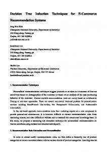
Decision Tree Example Interesting? Shape square

circle

Size

Color red

Yes

blue

No

triangle

large

green

Yes

Yes

No small

No

Interesting=Yes Ù ((Shape=circle)^((Color=red)V(Color=green))) V ((Shape=square)^(Size=large)) CSG220: Machine Learning

Decision Trees: Slide 2

1

Inducing Decision Trees from Data • Suppose we have a set of training data and want to construct a decision tree consistent with that data • One trivial way: Construct a tree that essentially just reproduces the training data, with one path to a leaf for each example • no hope of generalizing

• Better way: ID3 algorithm • tries to construct more compact trees • uses information-theoretic ideas to create tree recursively CSG220: Machine Learning


Inducing a decision tree: example • Suppose our tree is to determine whether it’s a good day to play tennis based on attributes representing weather conditions • Input attributes Attribute Outlook

Possible Values Sunny, Overcast, Rain

Temperature Hot, Mild, Cool Humidity

High, Normal

Wind

Strong, Weak

• Target attribute is PlayTennis, with values Yes or No CSG220: Machine Learning


2

Training Data

CSG220: Machine Learning


Essential Idea • Main question: Which attribute test should be placed at the root? • In this example, 4 possibilities • Once we have an answer to this question, apply the same idea recursively to the resulting subtrees • Base case: all data in a subtree give rise to the same value for the target attribute • In this case, make that subtree a leaf with the appropriate label CSG220: Machine Learning


3

• For example, suppose we decided that Wind should be used as the root • Resulting split of the data looks like this: Wind Strong

Weak

D2, D6, D7, D11, D12, D14

D1, D3, D4, D5, D8, D9, D10, D13

PlayTennis: 3 Yes, 3 No


• Is this a good test to split on? Or would one of the other three attributes be better? CSG220: Machine Learning


Digression: Information & Entropy • Suppose we want to encode and transmit a long sequence of symbols from the set {a, c, e, g} drawn randomly according to the following probability distribution D: Symbol

a

c

e

g

Probability

1/8

1/8

1/4

1/2

• Since there are 4 symbols, one possibility is to use 2 bits per symbol • In fact, it’s possible to use 1.75 bits per symbol, on average • Can you see how? CSG220: Machine Learning


4

• Here’s one way:

Symbol

Encoding

a

000

c

001

e

01

g

1

• Average number of bits per symbol =⅛*3+⅛*3+¼*2+½*1 = 1.75 • Information theory: Optimal length code assigns log2 1/p = - log2 p bits to a message having probability p CSG220: Machine Learning


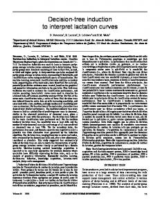
Entropy • Given a distribution D over a finite set, where are the corresponding probabilities, define the entropy of D by H(D) = - ∑i pi log2 pi • For example, the entropy of the distribution we just examined, , is 1.75 (bits) • Also called information • In general, entropy is higher the closer the distribution is to being uniform CSG220: Machine Learning


5

• Suppose there are just 2 values, so the distribution has the form • Here’s what the entropy looks like as a function of p:



Back to decision trees - almost • Think of the input attribute vector as revealing some information about the value of the target attribute • The input attributes are tested sequentially, so we’d like each test to reveal the maximal amount of information possible about the encourages shallower target attribute value Thistrees, we hope • To formalize this, we need the notion of conditional entropy



6

• Return to our symbol encoding example: Symbol

a

c

e

g

Probability

1/8

1/8

1/4

1/2

• Suppose we’re given the identity of the next symbol received in 2 stages: • we’re first told that the symbol is a vowel or consonant • then we learn its actual identity

• We’ll analyze this 2 different ways CSG220: Machine Learning


• First consider the second stage – conveying the identity of the symbol given prior knowledge that it’s a vowel or consonant • For this we use the conditional distribution of D given that the symbol is a vowel Symbol Probability

a

e

1/3

2/3

and the conditional distribution of D given that the symbol is a consonant Symbol Probability CSG220: Machine Learning

c

g

1/5

4/5 Decision Trees: Slide 14

7

• We can compute the entropy of each of these conditional distributions: H(D|Vowel) = - 1/3 log2 1/3 – 2/3 log2 2/3 = 0.918 H(D|Consonant) = - 1/5 log2 1/5 – 4/5 log2 4/5 = 0.722 • We then compute the expected value of this as 3/8 * 0.918 + 5/8 * 0.722 = 0.796 CSG220: Machine Learning


• H(D|Vowel) = 0.918 represents the expected number of bits to convey the actual identity of the symbol given that it’s a vowel • H(D|Consonant) = 0.722 represents the expected number of bits to convey the actual identity of the symbol given that it’s a consonant • Then the weighted average 0.796 is the expected number of bits to convey the actual identity of the symbol given whichever is true about it – that it’s a vowel or that it’s a consonant



8

Information Gain • Thus while it requires an average of 1.75 bits to convey the identity of each symbol, once it’s known whether it’s a vowel or a consonant, it only requires 0.796 bits, on average, to convey its actual identity • The difference 1.75 – 0.796 = 0.954 is the number of bits of information that are gained, on average, by knowing whether the symbol is a vowel or a consonant • called information gain CSG220: Machine Learning


• The way we computed this corresponds to the way we’ll apply this to identify good split nodes in decision trees • But it’s instructive to see another way: Consider the first stage – specifying whether vowel or consonant • The probabilities look like this: Probability

Vowel

Consonant

3/8

5/8

• The entropy of this is - 3/8 * log2 3/8 – 5/8 * log2 5/8 = 0.954 CSG220: Machine Learning


9

Now back to decision trees for real • We’ll illustrate using our PlayTennis data • The key idea will be to select as the test for the root of each subtree the one that gives maximum information gain for predicting the target attribute value • Since we don’t know the actual probabilities involved, we instead use the obvious frequency estimates from the training data • Here’s our training data again: CSG220: Machine Learning


Training Data



10

Which test at the root? • We can place at the root of the tree a test for the values of one of the 4 possible attributes Outlook, Temperature, Humidity, or Wind • Need to consider each in turn • But first let’s compute the entropy of the overall distribution of the target PlayTennis values: There are 5 No’s and 9 Yes’s, so the entropy is - 5/14 * log2 5/14 – 9/14 * log2 9/14 = 0.940 CSG220: Machine Learning


Wind Strong

Weak

D2, D6, D7, D11, D12, D14

D1, D3, D4, D5, D8, D9, D10, D13



H(PlayTennis|Wind=Strong) = - 3/6 * log2 3/6 - 3/6 * log2 3/6 = 1 H(PlayTennis|Wind=Weak) = - 6/8 * log2 6/8 - 2/8 * log2 2/8 = 0.811 So the expected value is 6/14 * 1 + 8/14 * 0.811 = 0.892 Therefore, the information gain after the Wind test is applied is 0.940 – 0.892 = 0.048



11

• Doing this for all 4 possible attribute tests yields Attribute tested at root

Information Gain

Outlook

0.246

Temperature

0.029

Humidity

0.151

Wind

0.048

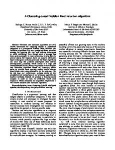
• Therefore the root should test for the value of Outlook CSG220: Machine Learning


Partially formed tree Entropy here is -2/5 log2 2/5 – 3/5 log2 3/5 = 0.971

Correct test for here among Temperature, Humidity, and Wind is the one giving highest information gain with respect to these 5 examples only


This node is a leaf since all its data agree on the same value


12

The Fully Learned Tree



Representational Power and Inductive Bias of Decision Trees • Easy to see that any finite-valued function on finite-valued attributes can be represented as a decision tree • Thus there is no selection bias when decision trees are used • makes overfitting a potential problem

• The only inductive bias is a preference bias: roughly, shallower trees are preferred CSG220: Machine Learning


13

Extensions • Continuous input attributes • Sort data on any such attribute and try to identify a high information gain threshold, forming binary split

• Continuous target attribute • Called a regression tree – won’t deal with it here

• Avoiding overfitting

More on this later

• Use separate validation set • Use tree post-pruning based on statistical tests



Extensions (continued) • Inconsistent training data (same attribute vector classified more than one way) • Store more information in each leaf

• Missing values of some attributes in training data • See textbook

• Missing values of some attributes in a new attribute vector to be classified (or missing branches in the induced tree) • Send the new vector down multiple branches corresponding to all values of that attribute, then let all leaves reached contribute to result CSG220: Machine Learning


14