colic, credit-a, credit-g, diabetes, glass, heart-c, heart-h, heart-statlog, hepatitis, ionosphere, iris, kr-vs-kp, labor, letter, lymph, mushroom, primary-tumor, segment ...
A Clustering-based Decision Tree Induction Algorithm Rodrigo C. Barros, Andr´e C. P. L. F. de Carvalho Department of Computer Science, ICMC University of S˜ao Paulo (USP) S˜ao Carlos - SP, Brazil {rcbarros,andre}@icmc.usp.br
Abstract—Decision tree induction algorithms are well known techniques for assigning objects to predefined categories in a transparent fashion. Most decision tree induction algorithms rely on a greedy top-down recursive strategy for growing the tree, and pruning techniques to avoid overfitting. Even though such a strategy has been quite successful in many problems, it falls short in several others. For instance, there are cases in which the hyper-rectangular surfaces generated by these algorithms can only map the problem description after several sub-sequential partitions, which results in a large and incomprehensible tree. Hence, we propose a new decision tree induction algorithm based on clustering which seeks to provide more accurate models and/or shorter descriptions more comprehensible for the end-user. We do not base our performance analysis solely on the straightforward comparison of our proposed algorithm to baseline methods. Instead, we propose a data-dependent analysis in order to look for evidences which may explain in which situations our algorithm outperforms a well-known decision tree induction algorithm. Keywords-decision trees; clustering; hybrid intelligent systems; data-dependency analysis; machine learning
I. I NTRODUCTION Classification is a supervised learning task that assigns objects to predefined categories. It has been widely studied and employed in intelligent decision making. A vast amount of works proposed by researchers in machine learning and statistics in the last decades have investigated new classification algorithms for general or domain-specific tasks. Decision tree induction algorithms are a subgroup of methods for classification that provide a hierarchical tree representation of the induced knowledge. Such a representation is intuitive and easy to assimilate by humans, which partially explains the large number of studies that make use of these techniques. Some well-known algorithms for decision tree induction are C4.5 [1] and CART [2]. Whilst the most successful decision tree induction algorithms employ a top-down recursive strategy for growing the trees, more recent works have opted for more efficient strategies. For instance, creating an
M´arcio P. Basgalupp, Marcos G. Quiles Instituto de Ciˆencia e Tecnologia Universidade Federal de S˜ao Paulo (UNIFESP) S˜ao Jos´e dos Campos - SP, Brazil {basgalupp,quiles}@unifesp.br
ensemble of trees is a growing topic at the machine learning community, especially because of the accurate models obtained in several experiments. Ensembles are created by inducing different decision trees from training samples and the ultimate classification is generally given through a voting scheme. Part of the research community avoid the ensemble solution with the argument that the comprehensibility component of analyzing a single decision tree is lost. Indeed, classification models being combined in an ensemble are often inconsistent with each other. Note that this inconsistency is necessary to achieve diversity in the ensemble, which in turn is necessary to increase its predictive accuracy [3]. Since comprehensibility may be crucial in several applications, ensembles are usually not a good option for these cases. Another approach that has been increasingly used is the induction of decision trees through Evolutionary Algorithms (EAs). The main benefits of evolving decision trees are the EAs’ capability of escaping local optima. EAs perform a robust global search in the space of candidate solutions, and thus they are less susceptible to local optima convergence. In addition, as a result of this global search, EAs tend to cope better with feature interactions than greedy methods, which means that complex feature relationships which are not detected during the greedy evaluation can be discovered by an EA that evolves decision trees [4]. The main disadvantages of evolutionary induction of decision trees are related to time and space constraints. EAs are a solid but computational expensive heuristic. Another disadvantage lies on the large number of parameters that need to be set (and tuned) in order to optimally run the EA for decision tree induction. As with every machine learning algorithm developed to date, there are pros and cons in using one strategy or another for decision tree induction. Moreover, algorithms that excel in a certain data set may perform poorly in others (i.e., the NFL theorem [5]). Whereas there are many studies that propose new classification algorithms every year, most of them
neglect the fact that the performance of the induced classifiers is heavily data dependent. Furthermore, these works usually present only superficial analyses that do not indicate the cases in which the proposed classifier may present significant gain over others. In an attempt to improve the accuracy of typical decision tree induction algorithms, and at the same time trying to preserve model comprehensibility, we propose a new classification algorithm based on clustering, named Clus-DTI (Clustering for improving Decision Tree Induction). The key insight that is exploited in this paper is that a difficult problem can be decomposed into much simpler sub-problems. Our hypothesis is that we can use clustering for improving classification with the premise that, instead of directly solving a difficult problem, independently solving its sub-problems may lead to improved performance. We investigate the performance of Clus-DTI regarding the data it is being applied to. Our contributions are twofold: (i) we propose a new classification algorithm whose objective is to improve decision tree classification through the use of clustering, and we empirically analyze its performance in public data sets; (ii) we investigate scenarios in which the proposed algorithm is a better option than a traditional decision tree induction algorithm. This investigation is based on data-dependency analyses. For such, it takes into account how the underlying data structure affects the performance of Clus-DTI. This paper is organized as follows. In Section II we detail the proposed algorithm, which combines clustering and decision trees. In Section III we conduct a straightforward comparison between Clus-DTI and the traditional decision tree induction algorithm C4.5 [1] (more specifically, its Java version, J48). Section IV presents a data-dependency analysis, where we suggest some scenarios in which Clus-DTI can be a better option than other algorithms. Section V presents studies related to our approach. We discuss the main conclusions of this study in Section VI. II. C LUS -DTI We have developed a new algorithm, named Clus-DTI (Clustering for improving decision tree induction), whose objective is to cluster the original classification data set in order to improve decision tree induction. It works based on the following premise: some classification problems are quite difficult to solve; thus, instead of growing a single tree to solve a potentially difficult classification problem, clustering the data set into smaller sub-problems may ease the complexity of solving the original problem. Formally speaking, our algorithm approximates the target function in specific regions of the input space,
instead of using the full input space. These specific regions are not randomly chosen, but defined through a well-known clustering strategy. It is reasonable to suppose that examples drawn from the same class distribution can be grouped together in order to make the classification problem simpler. We do not assume, however, that we can achieve a perfect cluster-to-class mapping (and we do not mean to). Our hypothesis is that solving sub-problems independently from each other, instead of directly trying to solve the larger problem, may provide better classification results overall. This assumption is not new and has motivated several strategies in computer science (e.g., the divide-and-conquer strategy). Clus-DTI combines two algorithms in order to generate classification models. It works as follows. 1) Given a classification training set X, Clus-DTI clusters X in p partitions Pi of i + 1 non-overlapping subsets of X, 1 ≤ i ≤ p, such that the first partition has two clusters, the second has three, the third has four, and so on. For example, partition P1 = {C1 , C2 }, and on a general form, Pi = {C1 , ..., Ci+1 }. In addition, Cj ∩ Ck = ∅ for j 6= k and C1 ∪ ... ∪ Ci+1 = X. In this step, Clus-DTI uses the well-known Expectation Maximization algorithm (EM) [6]. Since it is a statistical clustering method where all examples belong to all clusters with a given probability, it will assign each example to the most-probable cluster (hard assignment). Clus-DTI ignores the target feature when clustering the training set. 2) Once all examples are assigned to a cluster, Clus-DTI builds a distinct decision tree to each cluster according to its respective data. It uses the well-known C4.5 decision tree induction algorithm [1]. Therefore, partition Pi will have a set of i + 1 distinct decision trees, D = {Dt1 , ..., Dti+1 }, trained according to data belonging to each one of the clusters. 3) In order to decide which partition will be selected among the p available ones, Clus-DTI offers two choices. The first one is evaluating each partition through the Simplified Silhouette Width Criterion (SSWC) [7], a well-known clustering validity criterion. The partition to be selected is the one that maximizes SSWC, which implies minimizing the intra-group dissimilarity while maximizing the inter-group dissimilarity. The dissimilarity measure we have used in this work is the Mahalanobis distance [8], since the clusters produced by this crisp version of EM will most likely have an ellipsoidal shape. The second option is simpler and straightforward: choosing the number of clusters of the partition that maximizes training accuracy. Since we are dealing with a classification problem, perhaps the best option for choosing an ideal number of clusters is through
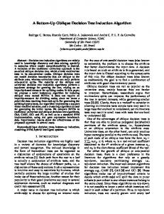
Training Data
Clustering
p partitions
Selection Criterion
k clusters
Generate DTs
Data Cluster each instance and classify it according to the corresponding DT Testing Data
k DTs
Final Classification
Figure 1.
Clus-DTI scheme.
a classification criterion, and accuracy is the most well-known evaluation measure for classification. 4) After partition Pi has been chosen, each example belonging to the test set Z is assigned to one of the i+1 clusters, and the corresponding decision tree Dtk , 1 ≤ k ≤ i + 1 is used to classify the test example. This procedure is repeated to every example in test set Z. Figure 1 depicts the previously mentioned steps of Clus-DTI. A given partition, selected either by SSWC or training accuracy, generates k decision trees (built over the training data belonging to each of the k clusters). Next, each example belonging to the test set is assigned to the cluster whose gaussian is more likely to have produced it. The tree corresponding to the cluster whose example was assigned to is then used to classify that example. Note that we do not necessarily expect a full adherence of clusters to classes. While clustering the training data may sometimes gather examples from the same class in their own cluster, which would mean EM was capable of discovering the correct probability distribution parameters of a given class, we do not believe that would be the case for most real-world classification problems. Our intention on designing Clus-DTI was to provide subsets of data in which the classification problem is easier than the one of the original set. In other words, we want to identify situations in which the sum of the performance of decision trees in subsets results in better overall performance than the one of a single decision tree in the original set. Even though this concept may be similar to the one of an ensemble of trees, we do not make use of any voting scheme for combining predictions. The absence of a voting scheme results in an important advantage of Clus-DTI over ensembles: we can track which decision tree was used to achieve the prediction of a particular object, instead of relying on averaged results provided by inconsistent models.
III. B ASELINE C OMPARISON We tested the performance of Clus-DTI into 29 public UCI data sets [9] and compared it to the performance of J48 (java implementation of C4.5, available at the Weka Toolkit [10]). The data sets selected are: anneal, audiology, autos, balance-scale, breast-cancer, breast-w, colic, credit-a, credit-g, diabetes, glass, heart-c, heart-h, heart-statlog, hepatitis, ionosphere, iris, kr-vs-kp, labor, letter, lymph, mushroom, primary-tumor, segment, sick, sonar, soybean, vote and waveform-5000. Those data sets with k classes, k > 2, were transformed into k data sets with two classes (one class versus all other classes), so every classification problem in this paper is binary. The restriction of dealing only with binary classification problems is due to the fact that the geometrical complexity measures [11], [12] used in this study for data-dependency analyses can deal with only two classes in most cases. With the transformations, the 29 data sets became 156 data sets, which were divided as follows: 70% for training and 30% for testing. Table I presents the results obtained in this comparison between Clus-DTI and J48. # Wins indicates the number of data sets in which each method has outperformed the other regarding test accuracy. Largest (Average/Smallest) Difference is the greatest (average/smallest) difference in accuracy between methods when one of them outperformed the other. Difference ≥ x% is the number of data sets in which a method has achieved a difference larger or equal than x% in terms of accuracy. We can notice that both methods are very similar in terms of number of times one outperforms the other (regarding accuracy). There were 83 ties, which were omitted. Clus-DTI outperformed J48 more often than not, suggesting the potential of clustering data sets. However, a non-parametric test such as the Wilcoxon Signed Rank Test [13] does not point out a statistically significant difference between the algorithms. Considering that Clus-DTI is computationally more costly than J48, it could be unwise to suggest choosing it over J48 for any problem. Thus, our goal is to investigate in which situations each algorithm is superior to the other and try to relate them to meta-data and measures of geometrical complexity of data sets. This discussion is presented in the next section. IV. D ATA - DEPENDENCY A NALYSIS It is often said that the performance of a classifier is data dependent [14]. Notwithstanding, works that propose new classifiers usually neglect data-dependency when analyzing their performance. The strategy usually employed is to provide a few cases in which the proposed classifier outperforms
Table I C OMPARISON BETWEEN C LUS -DTI AND J48.
# Wins Largest Difference Average Difference Smallest Difference Difference ≥ 1% Difference ≥ 3% Difference ≥ 5% Difference ≥ 7% Difference ≥ 10%
J48 34 8.88% 1.82% 0.8% 14 10 6 2 0
Clus-DTI 39 10% 1.84% 0.01% 19 5 2 1 1
baseline classifiers according to some performance measure. Similarly, theoretical studies that analyze the behavior of classifiers also tend to neglect data-dependency. They end up evaluating the performance of a classifier in a wide range of problems, resulting in weak performance bounds. Recent efforts have tried to link data characteristics to the performance of different classifiers in order to build recommendation systems [14]. Meta-learning is an attempt to understand data a priori of executing a learning algorithm. Data that describe the characteristics of data sets and learning algorithms are called meta-data. A learning algorithm is employed to interpret these meta-data and suggest a particular learner (or ranking a few learners) in order to better solve the problem at hand. Meta-learners for algorithm selection usually rely on data measures limited to statistical or information theoretic descriptions. Whereas these descriptions can be sufficient for recommending algorithms, they do not explain the geometrical characteristics of the class distributions, i.e., the manner in which classes are separated or interleaved, a critical factor for determining classification accuracy. Hence, geometrical measures are proposed in [11], [12] for characterizing the geometrical complexity of classification problems. The study of these measures is a first effort to better understand classifiers’ data-dependency. Moreover, by establishing the difficulty of a classification problem quantitatively, several studies in classification can be carried out, such as algorithm recommendation, guided data pre-processing and design of problem-aware classification algorithms. In this section, we make use of the previously mentioned meta-data and also of the measures proposed in [11], [12] to estimate the characteristics and geometrical complexity of several classification data sets. But first, we present a summary of the meta-data and geometrical measures we use to assess classification difficulty.
A. Meta-data The first attempt to characterize data sets for evaluating the performance of learning algorithms was made by Rendell et al. [15]. Their approach intended to predict the execution time of classification algorithms through very simple meta-features, such as number of features and number of examples. A significant improvement of such an approach was project STATLOG [16], which investigated the performance of several learning algorithms over more than twenty data sets. Approaches that followed deepened the analysis of the same set of meta-features for data characterization [17], [18]. This set of meta-features was divided in three categories: (i) simple; (ii) statistical; and (iii) information theory based. A more comprehensive set of meta-features is further discussed in [19]. We make use of the following measures presented in [19]: (1) number of examples; (2) number of features; (3) number of continuous features; (4) number of nominal features; (5) number of binary features; (6) number of classes; (7) percentage of missing values; (8) class entropy; (9) mean feature entropy; (10) mean feature Gini; (11) mean mutual information of class and features; and (12) uncertainty coefficient. In addition, we also used of the ratio of the number of examples of the less-frequent class to the most frequent class. For binary classification problems, it indicates the balancing level of the data set. Values closer to 1 indicate a balanced data set whereas values closer to 0 indicate an imbalanced data set. B. Geometrical complexity measures In [11], [12], a set of measures able to characterize data sets with regard to their geometrical structure is presented. These measures are divided intp three categories: (i) measures of overlaps in the feature space (OFS); (ii) measures of class separability (CS); and (iii) measures of geometry, topology, and density of manifolds (GTD). Table II presents a summary of them. C. Results of the data-dependency analysis We have calculated the 13 complexity measures and the 13 meta-features for the 156 data sets, and we have built a training set in which each example corresponds to a data set and each feature is one of the 26 measures. In addition, we have included the accuracy for J48 and the one for Clus-DTI, as well as the chosen k value of clusters and which method was better for each data set regarding accuracy (Clus-DTI, J48 or Tie). Thus, we have a training set of 156 examples and 30 features. Our intention with this training set is to perform a descriptive analysis in order to understand which aspects of the data have a higher influence in determining the performance of the algorithms. In
Table II S UMMARY OF THE GEOMETRICAL COMPLEXITY MEASURES . Measure
Description
F1 (OFS)
Computes the 2-class Fisher’s criterion. A high value of the measure indicates that there exists a vector that can separate examples belonging to different classes after these instances are projected on it. Computes the overlap of the tails of distributions defined by the examples of each class. A low value of F2 means that the features can discriminate well the examples of different classes. Computes the discriminative power of individual features, returning the value of the feature that discriminates the largest number of examples. A problem is easy if there exists one feature for which the ranges of values spanned by each class do not overlap. Follows the same idea presented by F3, but now it considers the discriminative power of all features. It returns the proportion of examples that have been discriminated, giving an idea of the fraction of instances whose class could be correctly predicted. Provides an estimate of the length of the class boundary. High values of this measure indicate that the majority of the examples lay closely to the class boundary, and so, that it may be more difficult for the learner to define this class boundary accurately. Compares the within-class spread with the distances to the nearest neighbors of other classes. Low values suggest that examples of the same class lay closely in the feature space. High values indicate that the examples of the same class are disperse. Denotes how close the examples of different classes are. It returns the leave-one-out error rate of the one-nearest neighbor (the kNN classifier with k=1) learner. Low values of this metric indicate that there is a large gap in the class boundary. Evaluates to what extent the data is linearly separable. It returns the sum of the difference between the prediction of a linear classifier and the actual class value. It returns zero for linearly separable problems. Provides information about to what extent the training data is linearly separable. It builds the linear classifier as explained in L1 and returns its training error. Given the data set, the method creates a test set by linear interpolation with random coefficients between pairs of random examples of the same class. L3 returns the test error rate of the linear classifier trained with the original data. Creates a test set as proposed by L3 and returns the test error of the 1NN classifier. It describes the shapes of class manifolds with the notion of adherence subset. An adherence subset is a sphere centered on an example of the data set which is grown as much as possible before touching any example of another class. T1 returns the number of spheres normalized by the total number of examples. Returns the ratio of the number of examples to the number of features. It is a rough indicator of sparseness of the data set.
F2 (OFS) F3 (OFS)
F4 (OFS)
N1 (CS)
N2 (CS)
N3 (CS)
L1 (CS)
L2 (CS) L3 (GTD)
N4 (GTD) T1 (GTD)
T2 (GTD)
particular, we search for evidences that may help the user to choose a priori the most suitable method for classification. First, we have built a decision tree over the previously described training set. The idea is that the rules extracted from this decision tree may offer an insight on the reasons one algorithm outperforms the other. In other words, we are using a decision tree as a descriptive tool instead of using it as a predictive tool. This is not unusual, since the classification model provided by the decision tree can serve as an explanatory tool to distinguish between objects of different classes [20]. Figure 2 shows this descriptive decision tree, which explains the behavior of roughly 85% of the training data. By analyzing the decision tree, we can infer that
Figure 2. Decision tree that describes the relationship between the measures and the most suitable algorithm to be used.
Clus-DTI is more robust regarding missing values than J48. A hypothesis that may explain this behavior is the fact that the number of missing values tend to be amortized among the clusters, and thus each tree that is built has to handle a smaller number of missing values. Another inference that can be made is regarding the remaining cases (those whose percentage of missing values is smaller than 8.21%) and measure T1. The reader should remember that measure T1 introduces the concept of adherence subsets. It grows hyperspheres that include examples from the same class and normalizes the count of hyperspheres to the total number of examples. The higher its value, the smaller the tendency of objects to be clustered in mono-class hyperspheres. The decision tree indicates that those cases in which the objects have a higher tendency of being clustered in mono-class hyperspheres (T 1 ≤ 0.865) are better handled by Clus-DTI. This seems to be a coherent conclusion since Clus-DTI clusters the data set in subsets, and the purer these subsets are, the easier the classification problem becomes. One potential problem in this analysis is that Clus-DTI does not generate clusters bounded by hyperspheres, but by hyper-ellipses. Nevertheless, this discovery seems to be valid even though our assumption is based on hyperspheres. For future work, we intend to modify T1 so it can grow hyper-ellipses
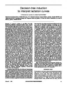
Figure 3. Bivariate analysis of F3 and number of features. Circles indicate the data sets in which Clus-DTI outperforms J48. Triangles indicate the data sets in which J48 outperforms Clus-DTI.
instead of hyperspheres. For the remaining cases (low percentage of missing values and high values of T1), the decision tree presents other relevant information. For instance, it tests the number of dimensions and also F3 (maximum feature efficiency). Figure 3 depicts the bivariate analysis of F3 and number of features. The lower rectangle indicates the first test over number of features separating those examples with less than 16 dimensions. The circles within the lower rectangle were already filtered by the decision tree during the tests over the percentage of missing values and T1. Therefore, the third test over number of features indeed separates the cases in which J48 outperforms Clus-DTI. The upper rectangle is the result of the fourth test, which is over the values of F3 (with the further restriction of having more than 16 dimensions, since the fourth test is a consequence of third test). Similar analyses can be performed with the remaining features of the decision tree. The next step is trying to understand the behavior of extreme cases, i.e., cases in which Clus-DTI achieves the highest and lowest differences in accuracy to J48. Tables III and IV present these cases, as well as some measures such as: (i) balance (ratio of the frequency of the less-frequent class to the most-frequent class), (ii) tree size of the tree generated by J48 in the full data set (Original TS), (iii) weighted-average of the tree size values from trees built for each cluster in Clus-DTI (Clus Average TS), (iv) accuracy achieved by J48 and (v) accuracy achieved by Clus-DTI. A careful analysis indicate that Clus-DTI performs better than J48 in imbalanced data sets (primary tumor and soybean). This is due to the fact that J48 generates a single leaf node for these data sets in which it
suggests the most frequent class, whereas Clus-DTI is able to explore the less-frequent class in its clusters. In the Soybean data set, for instance, Clus-DTI classifies correctly all examples from the rare class. Another interesting fact is that Clus-DTI generates smaller trees for all data sets (excluding the imbalanced data sets in which J48 builds a single node). This is predictable since we are reducing the size of the data set and, in some cases, eliminating several branches which would normally be built due to regions in which classes often overlap. Smaller trees present the advantage of being easier to interpret, besides of being more robust to overfitting than larger trees. Take the hepatitis data set, for example (not mentioned in Tables IV or III). Even though the difference between J48 and Clus-DTI is of 3.85% in favor of J48, Clus-DTI provides two distinct trees with 5 nodes each whereas J48’s single tree has 17 nodes. It is debatable which scenario the user would prefer to cope with: two small trees with 5 nodes each at the expense of 3.85% of accuracy or a large 17-node tree. It is clear that the number of victories of Clus-DTI should be adjusted to take into account a trade-off between accuracy and tree size. Thence, our last recommendation is for users for whom interpretability is a strong need: if none of the scenarios highlighted before suggested that Clus-DTI is a better option than J48, it may be still worthwhile using it due to the reduced size of the trees it generates. It should be noted that such an advantage disappears in those cases in which the number of clusters suggested by Clus-DTI multiplied by the average tree size of the clusters exceeds the tree size of J48’s single tree. V. R ELATED W ORK Very few works relate clustering and decision trees in the way we present in this paper. To the best of our knowledge, only one work presents some resemblance to our proposed algorithm, so we describe it next. Gaddam et al. [21] propose cascading K-Means and ID3 for improving anomaly detection. In their approach, the training data sets are clustered in k disjoint clusters (k is empirically defined) by the K-Means algorithm. A test example is first assigned to one of the generated clusters, and it is labeled according to the majority label of the cluster. An ID3 decision tree is built according to the training examples in each cluster (one tree per cluster) and it is also used for labeling the test example which was assigned to a particular cluster. The system also keeps track of the f nearest clusters from each test example, and it uses a combining scheme that checks for an agreement between K-Means and ID3 labeling. Whereas Clus-DTI shares a fair amount of similarities
Table III D ATA SETS IN WHICH C LUS -DTI OUTPERFORMS J48 BY LARGE MARGINS . Data set Audiology C2 Lymph C2 Primary Tumor C17 Soybean C12
Balance 0.3393 0.68 0.09 0.03
Original TS 11 15 1 1
Clus Average TS 8.14 7.28 2.43 9.53
K 2 3 6 2
Accuracy J48 96% 70% 91% 96%
Accuracy Clus 100% 80% 94% 100%
Table IV D ATA SETS IN WHICH J48 OUTPERFORMS C LUS -DTI BY LARGE MARGINS . Data set Autos C3 Heart-c C1 Heart-Statlog Ionosphere
Balance 0.47 0.83 0.8 0.56
Original TS 33 28 37 15
Clus Average TS 6.44 11.94 16.98 8.13
to the work of Gaddam et al., we highlight the main differences as follows: (i) Clus-DTI uses two different machine learning algorithms, EM and C4.5; (ii) Clus-DTI does not have a combining scheme for labeling test examples, which means our approach keeps its comprehensibility since we can directly track the rules responsible for labeling examples (which is not the case of the work in [21] and any other work that uses combining/voting schemes); (iii) Clus-DTI is not limited to anomaly detection applications; (iv) Clus-DTI automatically chooses the “ideal” number of clusters (from a predefined range) based on a clustering validity criterion; (v) Clus-DTI is conceptually simpler and easier to implement than K-Means+ID3, even though it makes use of more robust algorithms. VI. C ONCLUSIONS AND FUTURE WORK In this work, we have presented a new classification system which is based on the idea that clustering data sets may improve decision tree classification. Our algorithm, named Clus-DTI, makes use of well-known machine learning algorithms, namely Expectation Maximization [6] and C4.5 [1]. We have tested Clus-DTI using 29 public UCI data sets [9], which were transformed to binary class problems resulting in 156 distinct data sets. Experimental results indicated that Clus-DTI outperformed the baseline J48 algorithm more often than not, regarding accuracy. The difference, however, was not statistically significant according to the Wilcoxon Signed Rank Test [13]. A deeper analysis has been made in attempt to relate the underlying structure of the data sets with the performance of Clus-DTI. A total of 26 different measures were calculated to assess the complexity of each data set. Some of these measures were also used in classical meta-learning studies [17], [18].
K 2 4 3 2
Accuracy J48 79% 86% 82% 93%
Accuracy Clus 73% 80% 74% 87%
Other measures were suggested in more recent works [11], [12] in an attempt to assess data geometrical complexity. Through these measures, we were able to generate a decision tree for supporting a descriptive analysis whose goal was to point out scenarios in which Clus-DTI is a better option than J48 for data classification. We summarize our findings as follows: 1) Clus-DTI is quite robust to missing values. In fact, Clus-DTI outperformed J48 in all data sets whose percentage of missing values were above a certain threshold (8%). 2) The adherence subset concept is an important variable when choosing between algorithms. All cases in which the objects have a higher tendency of being clustered in mono-class hyperspheres (i.e., T 1 ≤ 0.865) were better handled by Clus-DTI. This seems to be coherent since we are clustering data a priori of classifying examples. Nevertheless, we would like to point out that the clusters produced by EM are bounded by hyper-ellipses and not hyperspheres. Reformulating T1 to grow hyper-ellipses may provide even better results. 3) Other important measures for helping the user to select the classification algorithm are number of features, maximum individual feature efficiency (F3) and the ratio of average intra/inter class nearest neighbor distance (N2). For the latter, it is intuitive to think that lower values of N2 - meaning that the classes are well-separated according to the euclidean distance - enhance the chances of Clus-DTI to provide better results, since it can group classes in different clusters, making the classification problem much easier. 4) Clus-DTI is robust to imbalanced classes. It achieved better results than J48 in all cases in which a single node is the resulting tree of J48. Clus-DTI reduces the impact of imbalanced classes when clustering them in different groups, eventually
finding the rules which describe the rare class. 5) J48 has performed better in 7 out of the 8 more-balanced data sets. This work is a first effort in the study of the potential benefits of clustering on classification. It presents a new classification algorithm that can also be seen as a framework that is more elegant than simply preprocessing data through clustering. It has opened several venues for future work, as follows. We intend to implement alternative methods of choosing the best value of k, such as calculating the accuracy of Clus-DTI over a validation data set and choosing the value of k that provides the best accuracy in that validation set. Also, we intend to test different clustering algorithms as well as different classification algorithms in our framework, in order to evaluate if our conclusions are generalizable for whichever pair of algorithms. Finally, we intend to test Clus-DTI in artificial data sets so we can guarantee its effectiveness in a variety of distinct scenarios, such as linearly-separable data, non-linearly separable data, imbalanced data sets, high-dimensional data, sparse data and other interesting problems. A CKNOWLEDGEMENT
[7] L. Vendramin, R. J. G. B. Campello, and E. R. Hruschka, “Relative clustering validity criteria: A comparative overview,” Stat. Anal. Data Min., vol. 3, pp. 209–235, August 2010. [8] P. C. Mahalanobis, “On the generalised distance in statistics,” in Proceedings National Institute of Science, India, vol. 2, no. 1, April 1936, pp. 49–55. [9] A. Frank and A. Asuncion, “UCI machine learning repository,” 2010. [Online]. Available: http://archive.ics.uci.edu/ml [10] I. H. Witten and E. Frank, Data Mining: Practical Machine Learning Tools and Techniques with Java Implementations. Morgan Kaufmann, October 1999. [11] T. K. Ho and M. Basu, “Complexity measures of supervised classification problems,” IEEE Trans. Pattern Anal. Mach. Intell., vol. 24, no. 3, pp. 289–300, 2002. [12] T. Ho, M. Basu, and M. Law, “Measures of geometrical complexity in classification problems,” in Data Complexity in Pattern Recognition. Springer London, 2006, pp. 1–23. [13] F. Wilcoxon, “Individual comparisons by ranking methods,” Biometrics, vol. 1, pp. 80–83, 1945.
Our thanks to Fundac¸a˜ o de Amparo a` Pesquisa do Estado de S˜ao Paulo (FAPESP) and Conselho Nacional ´ de Desenvolvimento Cient´ıfico e Tecnologico (CNPq) for supporting this research. Also, we would like to thank Dr. Alex A. Freitas for his valuable comments, which helped improving this paper.
[14] K. A. Smith-Miles, “Cross-disciplinary perspectives on meta-learning for algorithm selection,” ACM Comput. Surv., vol. 41, pp. 6:1–6:25, January 2009.
R EFERENCES
[16] D. Michie, D. J. Spiegelhalter, C. C. Taylor, and J. Campbell, Machine learning, neural and statistical classification. Ellis Horwood, 1994.
[1] J. R. Quinlan, C4.5: programs for machine learning. San Francisco, CA, USA: Morgan Kaufmann Publishers Inc., 1993. [2] L. Breiman, J. H. Friedman, R. A. Olshen, and C. J. Stone, Classification and Regression Trees. Wadsworth, 1984. [3] A. A. Freitas, D. C. Wieser, and R. Apweiler, “On the importance of comprehensible classification models for protein function prediction,” IEEE/ACM Transactions on Computational Biology and Bioinformatics, vol. 7, no. 1, pp. 172–182, 2010. [4] A. A. Freitas, Soft Computing for Knowledge Discovery and Data Mining. Springer US, 2008, ch. A Review of evolutionary Algorithms for Data Mining, pp. 79–111. [5] D. H. Wolpert and W. G. Macready, “No free lunch theorems for optimization,” IEEE Transactions on Evolutionary Computation, vol. 1, no. 1, pp. 67–82, 1997. [6] A. P. Dempster, N. M. Laird, and D. B. Rubin, “Maximum Likelihood from Incomplete Data via the EM Algorithm,” Journal of the Royal Statistical Society, vol. 39, no. 1, pp. 1–38, 1977.
[15] L. Rendell, R. Sheshu, and D. Tcheng, “Layered concept-learning and dynamically variable bias management,” in 10th international joint conference on Artificial intelligence, 1987, pp. 308–314.
[17] P. Brazdil, J. a. Gama, and B. Henery, “Characterizing the applicability of classification algorithms using meta-level learning,” in European Conference on Machine Learning, Secaucus, NJ, USA, 1994, pp. 83–102. [18] J. Gama and P. Brazdil, “Characterization of classification algorithms,” in 7th Portuguese Conference on Artificial Intelligence, London, UK, 1995, pp. 189–200. [19] A. Kalousis, “Algorithm selection via meta-learning,” Ph.D. dissertation, Universit´e de Gen`eve, Centre Universitaire d’Informatique, 2002. [20] P.-N. Tan, M. Steinbach, and V. Kumar, Introduction to Data Mining, (First Edition). Boston, MA, USA: Addison-Wesley Longman Publishing Co., Inc., 2005. [21] S. R. Gaddam, V. V. Phoha, and K. S. Balagani, “K-means+id3: A novel method for supervised anomaly detection by cascading k-means clustering and id3 decision tree learning methods,” IEEE Transactions on Knowledge and Data Engineering, vol. 19, pp. 345–354, 2007.