Decision Tree Pruning via Integer Programming ?
Yi Zhang Department of Management Sciences University of Iowa Iowa City, IA 52246, USA
Huang Huei-chuen Department of Industrial & System Engineering National University of Singapore 1 Engineering Drive 2, Singapore 117576
Abstract Decision tree is an important tool for classification in data mining. Many algorithms have been proposed to induce decision trees and most of them involve two phases, a growing phase and a pruning phase. In this paper, we concentrate on the pruning problem. We find that with the ultimate aim of selecting the best sub-tree with the minimal error for a separate test set, the problem can be formulated as an integer program with a nice structure. By exploiting the special structure of this integer program, we propose several interesting algorithms to identify the optimal sub-tree, including the one that is essentially the same as the well-known bottom-up pruning method with computational complexity of O(n). A new optimality proof of the above algorithm is provided from the perspective of mathematical programming. Key words: Data Mining, Decision Tree, Pruning, Optimization, Integer Program, Linear Program
? This research is supported by Singapore-MIT Alliance. Email addresses:
[email protected] (Yi Zhang),
[email protected] (Huang Huei-chuen).
Preprint submitted to Elsevier Science
17 August 2005
1
Introduction
Classification has been successfully used in many areas such as pattern recognition, medical diagnosis, and approval of loan application. Among the various techniques developed for classification, decision tree [5,2,9,1] is considered to be one of the most efficient one [6]. Usually a decision tree is built from a training set of data so that each of its leaf nodes is categorized as a certain class. To classify a new record, the attributes of this record are checked against the criterion associated with each internal node of the tree to determine the next successor node to be branched into. Finally the class to be received by the record is the class of the leaf node in which the record falls. Many algorithms have been proposed for inducing a good decision tree from a given database of records. Most of them involve two phases, a growing phase and a pruning phase. In the growing phase, a set of training data is used to determine the splits recursively. The growth stops when all the records in each of the branches belong to the same class or the number of records in each of the branches is sufficiently small. To have a more robust and reliable tree for predicting the classes of new records this overfitting tree is pruned at the second phase. A broad class of the common algorithms used in the pruning is the cost-complexity pruning [2,10] in which cost is imposed on the number of nodes that a tree has. By increasing the unit node cost, a sequence of subtrees with the minimal total cost of misclassification cost and node cost can be generated. A separate test set of data is then used to select from these candidates the best sub-tree with the minimal misclassification error out of the original overly grown tree. Besides cost-complexity pruning, a number of other pruning algorithms have been invented during the past decade such as reduced error pruning [10], pessimistic error pruning [10,11], minimum error pruning [3,8], critical value pruning [8], etc. It is clear that the aim of the pruning is to find the best sub-tree of the initially grown tree with the minimum error for the test set. However, the number of sub-trees of a tree is exponential in the number of its nodes and it is impractical computationally to search all the sub-trees. The main idea of the cost-complexity pruning is to limit the search space by introducing punishment on the number of nodes. There are questions on such simplification. While it is true that the tree size decides the variance-bias trade-off of the problem, it is questionable to apply an identical punishment weight on all the nodes. As the importance of different nodes may not be identical, it is foreseeable that the optimal sub-tree may not be included in the cost-complexity sub-tree candidates and hence it will not be selected. An interesting question to ask is whether there is an alternative good algorithm to identify the true optimal sub-tree. In this paper, it is found that the problem of searching for the optimal sub-tree can be formulated as an integer program. As the coefficient 2
matrix of the defining constraints satisfies the totally unimodular property, solving the integer program is equivalent to solving its relaxed linear program. In addition, the problem is found to resemble the problem of selecting a best subset of a given set and hence with a suitable reformulation the problem can be solved as a minimum cut problem via any network flow algorithm. Exploiting the structure of the problem further, we find that the problem can actually be solved by a combinatorial algorithm with computational complexity of O(n). This algorithm is essentially same as the “bottom-up” reduced error pruning procedure invented by Quinlan [10]. The contribution of this paper is to provide a new optimality proof of this efficient procedure. The remainder of the paper is organized as follows. In Section 2, we first give an integer program formulation for finding the optimal sub-tree. It is then followed by a better formulation as a problem of selecting a best subset out of a given set, along with a minimum cut algorithm to solve the problem. Finally we present a combinatorial algorithm with computational complexity of O(n) to identify the optimal sub-tree, as well as a new optimality proof based on primal-dual conditions. Section 3 concludes the paper.
2
Finding the Optimal Sub-tree
For simplicity, in this paper we present our analysis and results based on the framework used in CART [2] and in addition we assume that decision trees are binary. 2.1
An Integer Program for the Optimal Sub-tree
Assuming after the growing phase, a tree T has been built, with t0 as its root node. For each node tk of the tree, we assign a binary variable xk , xk =
1,
if the node belongs to the optimal subtree; 0, otherwise.
We also let the test set fall down the whole tree and calculate the respective misclassification cost ck for each node tk . In other words, if node tk is categorized as class j then ck =
X
C(i|j)Ni
i
where C(i|j) is the cost of misclassifying a record of class i as class j, and Ni equals the number of records of class i falling into node tk . 3
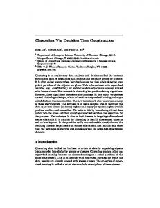
Fig. 1. A decision tree structure
For easiness of interpretation, we assign another variable yk to each node tk for the calculation of the overall misclassification cost in the objective function. The problem of searching for the best sub-tree with the minimum misclassification cost can be formulated as the following integer program: min x ,y i
i
X
ci yi
(1a)
i∈T
s.t. x0 = 1 xi = xj , ∀i, j ∈ tkc , ∀k ∈ T \ L xi ≥ xj , ∀j ∈ tic yi = xi − xj , ∀i ∈ T \ L, j ∈ ticl yi = xi , ∀i ∈ L xi ∈ {0, 1}, ∀i ∈ T
(1b) (1c) (1d) (1e) (1f) (1g)
where L represents the set of leaf nodes of the original tree, tic represents the set of direct child nodes of node ti , and ti cl represents the set consisting of the left child node of node ti. In the above integer program, constraint (1b) is imposed to ensure that the root node is selected. Constraint (1c) is imposed to ensure that both nodes belonging to the same parent node are chosen together or pruned together. Constraint (1d) is imposed to ensure that once child nodes are selected, their direct parent node must be selected as well. Constraint (1e) is imposed to ensure that for each child-parent node group, if the child nodes are chosen, the misclassification cost of the parent node will not be counted in the objective function. Constraint (1f) is imposed to ensure that if any of the original leaf nodes is chosen, its misclassification cost will be counted. It is clear that variables yi are not essential in the formulation and they can be eliminated by substitution. The simplified integer program is as follows, assuming that the original tree has a structure as shown in Figure 1. 4
min c0 x0 + (c1 − c0 )x1 + · · · + (cj − ci )xj + ck xk x i
+ cL2 xL2 + (cL3 − ck )xL3 + cL4 xL4 + · · · s.t. x0 = 1 x0 − x1 ≥ 0 ··· xi − xj ≥ 0 xj − xk = 0 xj − xL1 ≥ 0 xL1 − xL2 = 0 xk − xL3 ≥ 0 xL3 − xL4 = 0 ··· xi ∈ {0, 1}, ∀i ∈ T
2.2
(2a)
(2b)
Totally Unimodular Property of the Coefficient Matrix
Examining the second integer program, it is not difficult to see that the nonzero coefficient of each of its constraints has a value of either 1 or -1 and the coefficient matrix satisfies the sufficient condition stated in Proposition 1. Proposition 1 If the (0, 1, -1) matrix A has no more than two nonzero P entries in each row, and if j aij = 0 if row i contains two nonzero coefficients, then A is totally unimodular [7]. For a totally unimodular matrix, all the elements of the inverse matrix of any of its sub-squarematrix (if invertible) are integer. Therefore, the integer program has the same optimal solution as its relaxed linear program. In other words, we can replace the last constraint (2b) by the non-negativity constraint. As linear programs can be solved in polynomial time, the optimal sub-tree problem is also P-time solvable. Theorem 2 The optimal sub-tree problem can be solved in polynomial time.
2.3
Best Selection Formulation
The problem of selecting the best sub-tree resembles the problem of selecting the best subset nodes of a given set with a directed graph structure. The only difference is in its objective function, in which only the cost of part of 5
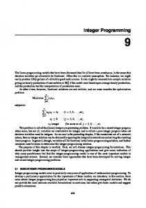
Fig. 2. An example decision tree with 14 nodes
the selected nodes is taken into account, i.e., the cost of the leaf nodes of the chosen sub-tree. However, this difference can be resolved by equating the cost of including a node as the coefficient associated with the respective node variables expressed in (2a). In other words, the cost can be modified according to the following rules: • • • •
The cost of the root node keeps unchanged. The cost of the right-child node remains unchanged. The cost of the left-child node equals the original cost of itself minus the original cost of its parent node.
For example, suppose a tree is grown as shown in Figure 2. The misclassification cost for the nodes are 100, 25, 35, 14, 19, 15, 21, 5, 8, 15, 11, 3, 18, 3, and 9 respectively. The modified cost for the nodes is given in Figure 3 in which the number in the bracket is its original cost and this number is present only when the original cost differs from the modified cost. To ensure that the selected set includes all the nodes of a sub-tree, a directed graph reflecting the parent-child and sibling relationships has to be constructed. For example, Figure 4 shows the graph for the above example in which the cost of each node has a reverse sign of its modified cost as the best selection problem is usually cast as a maximization problem. In the graph, the existence of the arrows is to ensure that if the node pointed is selected, the node pointing to it should also be selected. There is no arrow between the root node and the other part of the graph. This is because in order to select a non-empty sub-tree the root node must always be included. The rules for connecting the graph are: • No connection between the root node and the other part of the graph. • For the pair of parent and child nodes, the arrow points from the parent to 6
Fig. 3. The example decision tree with original and modified costs
Fig. 4. The example decision tree with best selection setup
the child. • For child nodes belonging to the same parent node, they are connected with a double-headed arrow.
2.4 A Minimum Cut for the Optimal Sub-tree
The best selection problem with an underlying network graph (V, A) and a weight function {wi } defined on the nodes can be viewed as a minimum cut problem [7]. To do this, we first add a source node s and a sink node t and 7
construct a new network graph as follows: V 0 = V ∪ {s, t}, A 0 = A ∪ A+ ∪ A − , A+ = {(i, t) : wi > 0, ∀i ∈ V }, A− = {(s, j) : wj ≤ 0, ∀j ∈ V }, c(i, t) = wi , ∀(i, t) ∈ A+ , c(s, j) = −wj , ∀(s, j) ∈ A− , c(i, j) = ∞, ∀(i, j) ∈ A.
From the definition of the cost function, it is not difficult to see that Proposition 3 is true. Proposition 3 Let Γ ⊆ V 0 . Define Γ0 = Γ ∪ {t}, S 0 = V 0 \ Γ0 , wj+ = P P max(0, wj ), W (Γ) = i∈Γ wi , and C(S 0 : Γ0 ) = (i,j)∈(S 0 :Γ0 ) c(i, j), where (S 0 : Γ0 ) = {(i, j) : (i, j) ∈ A0 , i ∈ S 0 , j ∈ Γ0 }. Then i. Γ is a selection of set V if and only if C(S 0 : Γ0 ) < ∞. P ii. if Γ is a selection, C(S 0 : Γ0 ) = j∈V wj+ − W (Γ) . From the above proposition, we have W (Γ) =
X
wj+ − C(S 0 : Γ0 ).
(3)
wj+ − min C(S 0 : Γ0 ). 0 0
(4)
j∈V
Hence, max W (Γ) = Γ⊆V
X
(S :Γ )
j∈V
In other words, the best selection problem is the same as the problem of finding the minimum cut of the derived graph . For the example presented in Figure 4, the derived graph is shown in Figure 5. The scribble line in the graph shows the solution of the minimum cut problem. When we calculate the numerical value of the minimum cut, we get: C(S 0 : Γ0 ) = 9 + 35 + 21 + 11 + 9 + 4 + 12 = 101. Hence, W (Γ) =
X
wj+ − C(S 0 : Γ0 )
j∈V
= 75 + 11 + 20 + 9 + 4 + 12 + 18 − 101 = 48. 8
Fig. 5. Minimum cut solution for decision tree pruning
And the objective function of the best sub-tree problem equals c0 − W (Γ) = 100 − 48 = 52. Here, Γ = Γ0 \ {t} = {1, 2, 5, 6, 13, 14} . Theorem 4 The optimal sub-tree problem is essentially a best selection problem. Hence it can be solved as a network flow (minimum cut) problem.
2.5
A Combinatorial Algorithm for the Optimal Sub-tree
Examining the constraints defining the linear program for finding the optimal sub-tree, we find that the optimal solution to the linear program can be constructed iteratively.
2.5.1 Algorithm Description Procedure A shows a way to construct the optimal sub-tree. Procedure A (1) Start from the leaf nodes of the original tree. (2) At the current level, calculate the sum of the cost of the nodes that belong to the same parent node. If the sum is less than the cost of the parent node, change the cost of the parent node to this sum. Otherwise, prune away the child nodes and the sub-tree downward connected with them, if there is any. 9
Fig. 6. “Bottom-up” pruning, first level pruned
(3) After processing all the nodes of the same level, move one level up and do the same step as (2) till we get to the root of the tree. The resulting sub-tree from Procedure A is the optimal sub-tree we are looking for and the cost of the root node is the cost of the selected sub-tree. The following illustrates the procedure for the example shown in Figure 3. First, we compare the sum of the cost of leaf nodes and the cost of their corresponding parent nodes. We get:
c7 + c8 = 13 < c3 = 14, c9 + c10 = 26 > c4 = 19, c11 + c12 = 21 > c5 = 15, c13 + c14 = 12 < c6 = 21. Hence, nodes 9, 10, 11, and 12 should be pruned away and the cost of nodes 3 and 6 should be changed to 13 and 12 respectively. After the first step, the tree will be like what is shown in Figure 6. Continuing the algorithm, we will get the final tree shown in Figure 7, which is the same sub-tree we obtain in Section 2.4. As this algorithm needs to check all the nodes only once, the complexity of the algorithm is O(n). As noted before, Procedure A is very similar to the “bottom-up” reduced error pruning firstly described in [10]. However, we are able to provide an alternative optimality proof of this combinatorial algorithm. 10
Fig. 7. “Bottom-up” pruning, second level pruned
2.5.2
A Primal-Dual Proof of the Combinatorial Algorithm
The dual linear program associated with the linear program for finding the best sub-tree of a tree in Figure 1 can be formulated as follows:
max λ0
(5)
λ,µ
s.t. λ0 + µ01 ≤ c0 − µ01 + λ12 + µ13 ≤ c1 − c0 ··· − µij + λjk + µjL1 ≤ cj − ci − λjk + µkL3 ≤ ck λL1 L2 − µjL1 ≤ cL1 − cj − λL1 L2 ≤ cL2 λL3 L4 − µkL3 ≤ cL3 − ck − λL3 L4 ≤ cL4 ··· µ≥0 λ unrestricted in sign
(6)
To construct the optimal sub-tree or to prove that Procedure A yields the best sub-tree we begin with the whole tree. In other words, let
x0 = x1 = · · · = xi = · · · = xL1 = xL2 = 1. 11
If the solution is optimal, according to the complementary slackness we would have λ0 + µ01 = c0 − µ01 + λ12 + µ13 = c1 − c0 ··· − µij + λjk + µjL1 = cj − ci − λjk + µkL3 = ck λL1 L2 − µjL1 = cL1 − cj − λL1 L2 = cL2 λL3 L4 − µkL3 = cL3 − ck − λL3 L4 = cL4 ···
(7a) (7b) (7c) (7d) (7e) (7f) (7g) (7h)
Starting from the leaf nodes we first check whether the corresponding dual variable satisfies the non-negativity constraints. If the constraints are violated, we then modify the values of xi iteratively to get an optimal dual solution that satisfies both the non-negativity and complementary slackness conditions. And at the same time the optimal sub-tree or the optimal solution of the primal problem is obtained. Beginning from (7g) and (7h), we get µkL3 = ck − (cL3 + cL4 ). If ck ≥ cL3 + cL4 , then µkL3 ≥ 0, non-negativity is satisfied, and from (7d), (7g), (7h) we get −λjk = cL3 + cL4 . Here, −λjk corresponds to the modified cost of node k. On the other hand, if ck < cL3 + cL4 , then we have µkL3 < 0. In order to preserve the non-negativity constraints, we set xL3 = xL4 = 0, µkL3 = 0, − λL3 L4 = cL4 , and drop the second last complimentary slackness constraint (7g). From (7d), we get λjk = ck . What it implies is simply that nodes L3 and L4 are pruned away. This is exactly the second step of Procedure A. After applying the same step to all the leaf nodes, we then move one level up. Suppose L1 , L2 are kept and L3 , L4 are pruned, i.e., xL1 = xL2 = 1, and xL3 = xL4 = 0. In this case, equations (7c) ∼ (7f) still hold with µkL3 = 0. 12
Summing them up, we get µij = ci − (cL1 + cL2 + ck ). Next, we have to check whether µij is non-negative. This checking corresponds to the cost comparison in Procedure A. On the other hand, if all of the leaf nodes, L1 , L2 , L3 and L4 , are kept, then equations (7c) ∼ (7h) hold. Summing them up, we get: µij = ci − (cL1 + cL2 + cL3 + cL4 ). Again checking the sign of µij to determine the values of xi and xj is exactly the same as what we do in Procedure A. Continuing the steps repeatedly, in the end we will get a sub-tree whose primal and dual variables satisfy the respective constraints and complementary slackness. This means that the corresponding sub-tree is optimal. And these steps are essentially the same as those of Procedure A. Theorem 5 The optimal sub-tree problem has a combinatorial algorithm whose computational complexity is O(n).
2.5.3
Comparison of Optimal Pruning versus Cost Complexity Pruning
We give an example to show that the optimal pruning algorithm will render a better result than the one pruned by the cost-complexity. The context of the example is a three-class problem based on the convex combination of three basic waveforms. A detailed description of the example can be found in [2]. Figure 8 shows the leftmost part of the tree produced by the standard CART algorithm. The entire tree has 11 terminal nodes. The re-substitution estimate of the misclassification error rate is 0.14 and the estimate of misclassification error rate obtained by an independent test set of size 5000 is 0.28. Within each node in Figure 8 are the population sizes of the three classes of the node. The question inducing the split is indicated beneath each node. The numbers to the right of each node are the normalized counts of the population sizes of the three classes of the 5000 test samples. When we apply Procedure A to the tree, we find that there is still room for improvement. For example, consider the leftmost decision node of this tree. For the present tree, two leaf nodes are grown from the criterion x6 ≤ 0.8. They are labeled as class 3 and class 1 respectively. The test set error rates are 14/27 and 6/24 for the left and right leaf nodes respectively. The total error rate is 20/51. But if we prune these two nodes away and let their parent decision node be a leaf node, which should be labeled as class 1, we find that the test 13
Fig. 8. Pruned tree for waveform dataset
set error rate is 19/51, which is 1/51 less than the current tree. Therefore, judging from the test set error, in general Procedure A gives a better tree than the one obtained by the cost-complexity pruning. Given the fact that Procedure A will produce a tree with minimum test set error, it is still too early to conclude that Procedure A is a better pruning method than other ones. As a matter of fact, the “test set” in this paper should be called “tuning set” or “pruning set” and regarded as part of the training set, since it is used to modify the learning model. For a fair comparison of different pruning methods, a truly held-out evaluation set should be used to evaluate their performance. Since the integer program and the reduced error pruning method, which has been well studied, will give the same result, any previously drawn conclusion upon on the reduced error pruning method in terms of performance will apply to the algorithms presented in this paper. It is thus convenient for the author to refer to some empirical study literatures that conducted extensive computational experiments for comparison among different pruning algorithms, such as the work done by Quinlan [10] and Esposito et al. [4].
3
Conclusion
This paper formulates the decision tree pruning process as an integer optimization problem. We propose a few efficient algorithms to solve this integer program and the fastest among them has computational complexity of only O(n), where n is the number of the nodes of the original tree. Applying this model, we have also successfully improved an example produced by CART in 14
terms of test set error. Although the integer program proposed in this paper produce the same result as the reduced error pruning, it opens a new perspective onto the decision tree pruning problem. We hope that new ideas could be inspired by the interesting theoretical findings of this paper.
References
[1] K. P. Bennett. Decision tree construction via linear programming. In Proceedings of the 4th Midwest Artificial Intelligence and Cognitive Science Society Conference, pages 97–101, 1992. [2] L. Breiman, J. Friedman, R. Olshen, and C. Stone. Classification and Regression Trees. Wadsworth and Brooks, 1984. [3] B. Cestnik and I. Bratko. On estimating probabilities in tree pruning. In EWSL-91: Proceedings of the European working session on learning on Machine learning, pages 138–150, New York, 1991. Springer-Verlag. [4] F. Esposito, D. Malerba, and G. Semeraro. A comparative analysis of methods for pruning decision trees. IEEE Transactions on Pattern Analysis and Machine Intelligence, 19(5):476–491, 1997. [5] E. B. Hunt, J. Marin, and P. J. Stone. Experiments in Induction. Academic Press, 1966. [6] D. Mitchie, D. J. Spiegelhalter, and C. C. Taylor. Machine Learning, Neural and Statistical Classification. Ellis Horwood, 1994. [7] G. L. Nemhauser and L. A. Wolsey. Integer and Combinatorial Optimization. John Wiley & Sons, 1988. [8] T. Niblett and I. Bratko. Learning decision rules in noisy domains. Proceedings of Expert Systems 86. Cambridge University Press, 1986.
In
[9] J. R. Quinlan. Induction of decision trees. Machine Learning, 1(1):81–106, 1986. [10] J. R. Quinlan. Simplifying decision trees. In B. Gaines and J. Boose, editors, Knowledge Acquisition for Knowledge-Based Systems, pages 239–252. Academic Press, London, 1988. [11] R. J. Quinlan. C4.5: Programs for Machine Learning. Morgan Kaufman, San Manteo, CA, 1993.
15