Decomposing Global Quantitative Properties into Local Ones Ilaria Matteucci1 , Francesco Santini2 1
2
Istituto di Informatica e Telematica, IIT-CNR, Pisa, Italy
[email protected] Dipartimento di Matematica e Informatica, Universit` a di Perugia, Italy
[email protected]
Abstract. In this paper we address the problem of identifying what local properties the sub-components of a system have to satisfy in order to guarantee a (security) property on the behaviour of the whole system. We associate each action with a value. Hence, we end up with quantitative properties on them, which are specified through a modal logic equipped with a parametric algebraic structure (i.e., a c-semiring). The aim is to have a value related to the satisfaction of a formula. Starting from the behaviour of a general distributed system (or context), we propose a formal approach to decompose a global quantitative property into the local quantitative properties to be satisfied by its sub-contexts.
1
Introduction
Understanding, reasoning, and designing distributed systems can be problematic. As such systems grow in size and decentralisation degree, their development demands for rigorous formal approaches. An example is the verification of security properties, as which actions a component is allowed to perform at a given moment, depending upon what actions a different component has executed. For instance, let us consider the classical Chinese-Wall security-policy regulating the access to two sets of resources A and B, and a system that is a composition of two unknown components, both able to access to A and B. The global system satisfies the Chinese-Wall property if and only if the two components coordinate their actions in such a way that the system accesses to only one of the two sets; thus, if it is accesses to A, it cannot then access to B (and vice-versa). The goal of the paper is to describe a formal machinery that allows us to opportunely find out the properties that must be locally satisfied by each of the unknown components over their composition, to guarantee a given property (i.e., in this case, the Chinese-Wall policy). In addition to this, we consider quantitative aspects, in order to add to the picture costs, execution times, rates and, in general, other non-functional aspects. Therefore, the relevant question is not only whether a system verifies a boolean property (as a security feature), but also how much enforcing it impacts on other desiderata. This “how much” corresponds to a generic cost needed to verify that property, for instance by considering the cost of all the actions
required to satisfy it. In particular, the ultimate aim of this work is to identify the quantitative constraints each system subcomponents has to satisfy in order to allow the whole system to behave as expected (i.e., verifying a boolean property), and, at the same time, with a cost better than a user-defined threshold t. In the following, Sec. 2 presents the necessary background-notions about csemirings [2,3], the algebraic structure we use to parametrise different cost/preference metrics: anything that can be cast to a semiring is still usable in the same framework. In Sec. 3, we introduce the notion of quantitative contexts, i.e., contexts whose actions are associated with a c-semiring value. Contexts have been introduced in [10] with the purpose to formally specify and analyse generic distributed-systems. Section 4 and Sec. 5 represent the core of this work: there i) we recall and enhance a quantitative Hennessy-Milner logic (i.e., c-HM logic) [14] to define quantitative properties on n-ary context and ii) we provide all the necessary formal tools for decomposing quantitative properties satisfied by an n-ary context into n local ones, each of them satisfied by a unary (quantitative) context. Each context represents a different component of a distributed system. In Sec. 6 we sketch an example of a well-known security model, i.e., the Chinese-Wall, rephrased with security-levels and then decomposed. In this way we can observe i) whether the specified policy is classically respected, and ii) whether the contribution of each distributed component (in terms of the securitylevel of its actions) is enough to guarantee a minimum global-security. Finally, Sec. 7 reports the related work, and Sec. 8 presents conclusions and future work.
2
C-semirings
We introduce c-semirings, the core of the presented computational framework. Definition 1 (Semiring [8]). A commutative semiring is a five-tuple K “ xK, `, ˆ, K, Jy such that K is a set, J, K P K, and `, ˆ : K ˆ K Ñ K are binary operators making the triples xK, `, Ky and xK, ˆ, Jy commutative monoids (semigroups with identity), satisfying – (distributivity) @a, b, c P K.a ˆ pb ` cq “ pa ˆ bq ` pa ˆ cq. – (annihilator) @a P A.a ˆ K “ K. Definition 2 (Absorptive semirings). Let S be a commutative semiring. An absorptive semiring verifies the absorptiveness property: @a, b P K.a`paˆbq “ a, which is equivalent to @a P S.a ` J “ J. Absorptive semirings are referred as simple, and their ` operator is necessarily idempotent [8]. Semirings where ` is idempotent are tropical, or diods. Definition 3 (C-semiring [3]). C-semirings are commutative and absorptive semirings. Therefore, c-semirings are tropical semirings where J is an absorbing element for `.
The idempotency of ` leads to the definition of a partial ordering ďK over the set K (K is a poset). It is defined as a ďK b if and only if a ` b “ b, and ` finds their least upper bound in K. This intuitively means that b is “better” than a. Therefore, we can use ` as an optimisation operator and always choose the best available solution. Some more properties can be derived on c-semirings [3]: i) both ` and ˆ are monotone over ďK , ii) ˆ is intensive (i.e., a ˆ b ďK a), iii) ˆ is closed (i.e., a ˆ b P K), and iv) xK, ďK y is a complete lattice. K and J are respectively the bottom and top elements of such lattice. When also ˆ is idempotent, i) ` distributes over ˆ, ii) ˆ is the greaterřlower bound (glb, or [) of the lattice, and iii) xK, ďK y is a distributive lattice. denotes the set-wise extension of `. Some c-semiring instances are: boolean xtF , T u, _, ^, F , T y3 , fuzzy xr0, 1s, max, min, 0, 1y, bottleneck xR` Yt`8u, max, min, 0, 8y, probabilistic xr0, 1s, max, ˆ 0, 1y (or Viterbi semiring), weighted xR` Y t`8u, min, `, ˆ `8, 0y. Capped ˆ, operators stand for their arithmetic equivalent. Although c-semirings have been historically used as monotonic structures where to aggregate costs (and find best solutions), the need of removing values has raised in local consistency algorithms and non-monotonic algebras using constraints (e.g., , [2]). A solution comes from residuation theory [4], a standard tool on tropical arithmetic that allows for obtaining a division operator via an approximate solution to the equation b ˆ x “ a. Definition 4 (Division [2]). Let K be a tropical semiring. Then, K is residuated if the set tx P K | b ˆ x ď au admits a maximum for all elements a, b P K, denoted a ˜ b. Since a complete4 tropical-semiring is also residuated, all the classical instances of c-semiring presented above are residuated, i.e., each element in K admits an “inverse”, which is unique in case ďK is a total order. For instance, the unique “inverse” a ˜ b in the weighted semiring is defined as follows: # 0 if b ě a ˆ ě au “ a ˜ b “ mintx | b`x ˆ a´b if a ą b Definition 5 (Unique invertibility [2]). Let K be an absorptive, invertible semiring. Then, K is uniquely invertible iff it is cancellative, i.e., @a, b, c P A.paˆ c “ b ˆ cq ^ pc ‰ 0q ñ a “ b. Since all the previous examples of c-semirings (e.g., weighted or fuzzy) are cancellative, they are uniquely invertible as well. Furthermore, it is also possible to consider several optimisation criteria at the same time: the Cartesian product of c-semirings is still a c-semiring. Clearly, in this case the ordering induced by ` is partial, e.g., when we have xk1 , k2 y and xk3 , k4 y, and k1 ď k3 while k2 ě k4 . 3 4
Boolean c-semirings can be used to model crisp problems. K is complete if it is closed with respect to infinite sums, and the distributivity law holds also for an infinite number of summands [2].
3
Quantitative Contexts
The notion of context has been introduced in [10] as an expression describing the partial implementation of a system, CpX1 , . . . , Xn q, where C denotes the known part, and X1 , . . . , Xn are free variables representing the unknown ones. In this section, we enhance the definitions of context given in [10] by adding the notion of a weight associated with tuple of actions. This allows us to quantitatively specify and analyse the behaviour of a distributed system with some unknowns part, which have nevertheless to participate to the satisfaction of a quantitative global-property on the whole system. Definition 6 (Quantitative context). A quantitative context-system is a m structure C “ pxCnm yn,m , Act, K, xÑK n,m yn,m q where xCn yn,m is a set of n-tom tuple of n-to-m quantitative contexts; K “ xK, `, ˆ, K, Jy is a c-semiring; Act is a set of actions; Act0 “ Act Y t0u where 0 R Act is a distinguished no-action symbol, Actn0 is the set of tuples of n actions in Act0 , and ÑK n,m Ď m Cnm ˆppActn0 , KqˆpActm , KqqˆC is the quantitative transduction-relation for n 0 the n-to-m contexts satisfying pC, p˜ a, kq, p˜0, hq, Dq PÑK if and only if C “ D n,m and a ˜ “˜ 0 for all contexts C, D P Cnm ph, k P Kq, and xÑK y are n-to-m n,m n,m tuple of quantitative transduction-relation. ˜
pb,hq ÝÝÑ C 1 , leaving the indices For pC, p˜ a, kq, p˜b, hq, C 1 q PÑK n,m we usually write C Ý p˜ a,kq
of Ñ to be determined by the context. The informal interpretation is that the context C takes in input the set of actions a ˜ performed with a weight k, and it returns as output ˜b weighted by h, finally becoming C 1 . If a ˜ is 0 (i.e., no action) then the context produces an output without consuming any internal action; if ˜b is 0 then there is not any observable transition and we omit the vector of outputs; if both a ˜ and ˜b are equal to 0, then both the internal process and the external observer are not involved in the transduction. We compose contexts by means of two operations: composition and product. Definition 7 (Composition). Let C “ pxCnm yn,m , Act, K, xÑK n,m yn,m q be a quantitative context-system. A composition on C is a dyadic operation ˝ on conr texts such that, whenever C P Cnm and D P Cm , then D ˝ C P Cnr according to the following rule: p˜ b,hq
C ÝÝÝÑ C 1 p˜ a,kq
p˜ c,wq
D ÝÝÝÑ D1 p˜ b,hq
p˜ c,wq
D ˝ C ÝÝÝÑ D1 ˝ C 1 p˜ a,kq
where a ˜ “ xa1 , . . . , an y, ˜b “ xb1 , . . . , bm y and c˜ “ xc1 , . . . , cr y are vectors of actions, while k, h, w represent the weight associated to the vector af actions a ˜, ˜b, and c˜ respectively. The basic idea is that two contexts can be composed if the output of the first one (cfr. D) is exactly the same in terms of i) the tuple of performed actions, ii) its associated weight, with respect to the input of the second context (cfr.
C). In this way, the two contexts combine their actions in such a way that the transduction of the composed context takes the input of D and its weight as input, and it returns the output of C and its weight as output. To compose n independent processes through the same context C P Cnm we define an independent combination, referred as the product operator of n contexts 1 D1 ˆ . . . ˆ Dn , where Di P Cm , i “ 1, . . . , n and Di is an expansion of the i’th i subcomponent of C such that the cardinality m is exactly equal to the sum of each cardinality mi associated with contexts Di . Definition 8 (Product). Let C “ pxCnm yn,m , Act, K, xÑK n,m yn,m q be a context system. A product on C is a context operation ˆ, such that whenever C P Cnm m`s and D P Crs then C ˆ D P Cn`r . Furthermore the transduction for a context C ˆ D are fully characterized by the following rule: b,hq p˜
C ÝÝÝÑ C 1 p˜ a,kq
˜ pd,sq
D ÝÝÝÑ D1 p˜ c,wq
˜ p˜ bd,hˆsq
C ˆ D ÝÝÝÝÝÝÑ C 1 ˆ D1 p˜ ac ˜,kˆwq
where juxtaposition of vectors a ˜ “ xa1 , . . . , an y and c˜ “ xc1 , . . . , cr y is the vector a ˜c˜ “ xa1 , . . . , an , c1 , . . . , cr y, and juxtaposition of vectors ˜b “ xb1 , . . . , bm y and d˜ “ xd1 , . . . , ds y is the vector ˜bd˜ “ xb1 , . . . , bm , d1 , . . . , ds y. Note that the weight of the juxtaposition of two action vectors is just the ˆ of their weights. For sake of readability, in the following we will write the combined process CpD1 , . . . , Dn q as a shorthand for C ˝ pD1 ˆ . . . ˆ Dn q. Note that, since we consider asynchronous contexts, it is not required that all the components D1 , . . . , Dn contribute in a transition of the combined process CpD1 , . . . , Dn q, i.e., some Di can perform a 0 action.
4
Quantifying Properties in a Distributed Environment
In this section, we mainly focus on how we can express quantitative properties/constraints on distributed systems. To this aim, we propose a variant of a quantitative Hennessy-Milner logic, the c-HM logic firstly proposed in [14]; thus, we can specify a property on a tuple of actions, extending it to c-HMn . 4.1
Multi-action C-semiring Hennessy-Milner Logic (c-HMn )
We start by defining the transition system on which c-HMn is defined: Definition 9 (MLTS). A (finite) Multi-Labelled Transition-System (MLTS) is a five-tuple MLTS “ pS, Ln , K, T q, where i) S is the countable (finite) statespace, ii) Ln is a finite set of transition labels, where each label is a vector of labels in L: the label xa1 , . . . , an y P Ln and for all i “ 1, . . . , n, ai P L. iii) K “ xK, ď, ˆ, ˜, 1, K, Jy is an IReM used for the definition of transition weights, and iv) T : pS ˆ Ln ˆ Sq ÝÑ K is the transition weight-function.
JkKpCq Jφ1 \ φ2 KpCq Jφ1 ˆ φ2 KpCq Jφ1 [ φ2 KpCq Jxxa ˜y φKpCq Jrra ˜s φKpCq
m “ k P K @C P Cn “ Jφ1 KpCq \ Jφ2 KpCq “ Jφ1 KpCq ˆ Jφ2 KpCq “ Jφ1 KpCq [ Jφ2 KpCq Ů “ pka ˆ JφKpC 1 qq R Ű “ pka ˆ JφKpC 1 qq R
where R “ tC 1 P C0m | pC, p˜a, ka q, p0, Jq, C 1 q P T u Table 1. The semantic interpretation of c-HM. We have
ř Ű pHq “ K and pHq “ J.
Definition 10 syntactically defines the correct formulas given over an MLTS. Definition 10 (Syntax). Given an MLTS M “ xS, Ln , K, T y, and let a ˜ P Ln , the syntax of a formula φ P ΦM is as follows, where k P K: φ ::“ k | φ1 \ φ2 | φ1 ˆ φ2 | φ1 [ φ2 | x a ˜y φ | r a ˜s φ The operators \ and [ (respectively the lub and glb derived from ě in K), and ˆ (still in the definition of K) are used in place of classical logic operators _ and ^, in order to compose the truth values of two formulas together. Truth values are all the k P K. In particular, while false corresponds to K, we can have different degrees of true, where “full truth” is J. As a reminder, when the ˆ operator is idempotent, then ˆ and [ coincide (Sec. 2). Finally, we have the two classical modal operators, i.e., “possibly” (xx ¨ y ), and “necessarily” (rr ¨ s ). The semantics of a formula φ is interpreted on a system of quantitative K contexts, given on top of an MLTS M “ pCnm , Actn0 ˆ Actm 0 , K, Ñn,m q. The aim is to check the specification defined by φ over the behaviour of a weighted transition system M that defines the behaviour of a quantitative context. While in [10] the semantics of a formula computes the states U Ď Cnm that satisfy that formula, our semantics J KM : pΦM ˆ Cnm q ÝÑ K (see Tab. 1) computes a truth value for the same U . In particular, in the following we deal with n-ary contexts (C0n ), hence the set of labels is Ln “ Actn0 . Note that we consider finite contexts Cnm , i.e., they are defined over a finite MLTS, they are not recursive, and the contexts composed with them are closed and finite as well. In Tab. 1 and in the following (when clear from the context), we omit M from J KM for the sake of readability. The semantics is parametrised over a context C P Cnm , which is used to consider only the transitions that can be fired at a given step (labelled with a vector of actions a ˜). In Def. 11 we rephrase the notion of satisfiability of a c-HMn formula φ on a context C by taking into account a threshold t (t-satisfiability): Definition 11 ((t ). A context C P Cnm satisfies a c-HMn formula φ with a threshold-value t, i.e., C (t φ, if and only if the interpretation of φ on C is better/equal than t. Formally: C (t φ ô t ď JφKC .
This means that C is a model for a formula φ, with respect to a certain value t, if and only if the weight corresponding to the interpretation of φ on C is better or equal to t in the partial order ď defined in K. Remark 1. Note that, if C does not satisfy a formula φ then JφKC “ K. Consequently, the only t such that C (t φ is t “ K. If JφKC ‰ K, then φ is satisfiable with a certain threshold t ‰ K.
5
Decomposition of Properties
In this section we provide a machinery for decomposing quantitative properties satisfied by a context C0n , which can be written as the product of n C01 contexts, into local quantitative properties, each of them satisfied by such a unary context.5 Indeed, let CpX1 , . . . , Xn q be a distributed system, in which X1 , . . . , Xn are system subcomponents. We are interested in identifying which are the local properties or constraints, expressed by a logic formula c-HM1 , each Xi , i “ 1, . . . , n has to quantitatively satisfy that CpX1 , . . . , Xn q quantitatively satisfies a global property expressed by a n-ary logic formula in c-HMn . This satisfaction is given with respect to a threshold value t concerning a quantitative requirement on the evaluation of φ, which is required to be better than t P K. Formally, this can be expressed as @Xi , i “ 1, . . . , n
CpX1 , . . . , Xn q (t φ.
(1)
Due to the expressive power of c-HMn (see Sec. 4.1), we mainly consider safety properties, e.g., properties expressing that if something goes wrong it can be detected in a finite number of steps. In order to solve the problem in Eq. 1, we provide formal tools to simplify this problem by splitting φ into local properties to be projected on each unknown Xi i.e., the problem in Eq. 1 is reduced to a set of problems Xi (ti φi , @i P I, where Xi P C01 and φi and ti are the output of the decomposition procedure. In words, we decompose φ1 over the unknown parts. Similarly to [10], we define a n-tuple formula as a unary c-HMn formula represented as a vector of n components xφ1 , . . . , φn y, where each φ1 , . . . , φn is a closed and unary formula in c-HM1 . xφ1 , . . . , φn y is unary because we let its evaluation correspond to Jφ1 ˆ . . . ˆ φn K. Definition 12 (Tuple-formulas). xφ1 , . . . , φn y is an n-tuple formula where each φi , i “ 1, . . . , n is a unary formula such that, for the context X1 ˆ . . . ˆ Xn : Jxφ1 , . . . , φn yKpX1 ˆ . . . ˆ Xn q “ Jxφ1 yKpX1 q ˆ . . . ˆ Jxφn yKpXn q For a tuple formula φ, we say that φ is quantitatively weakly valid if it is satisfied by all the possible n-product contexts X1 ˆ . . . ˆ Xn , within a given quantitative context-system. Hereafter we focus on the decomposition of a formula φ into the components of a tuple-formula. To do this, we first introduce the notion of equality between 5
It is worth noting that this follows the notion of weakly validity introduced in [10].
two formulas i.e., φ1 “ φ2 , in such a way that the result is J if they are both evaluated to the same k P K, K otherwise. Formally, " J if Jφ1 KpCq “ Jφ2 KpCq. Jφ1 “ φ2 KpCq “ (2) K otherwise. Hence, the decomposition we need can be formally stated as the search for a single tuple formula xφ1 , . . . , φn y such that xφ1 , . . . , φn y “ φ is a tautology, i.e., Jxφ1 , . . . , φn y “ φKpCq “ J for any C. Therefore, we can state xφ1 , . . . , φn y is quantitatively weakly valid. Note that, according to the definition of “, this is equivalent to state that Jxφ1 , . . . , φn yKpCq “ JφKpCq for any C. Hereafter, when we use this notation we omit pCq for the sake of brevity. Usually there does not exist a single tuple formula that decomposes φ. Let φ be finite, there exists a finite collection of tuple formulas xφi1 , . . . , φin yiPI , for n finite collections of unary closed formulas xφij yiPI (I is a finite indexes set) s.t. ÿ
xφi1 , . . . , φin y “ φ
(3)
iPI
is a tautology (see Eq. 2). For the sake of clarity and simplicity, we curb to ř consider the decomposition of φ into 2-tuple formulas, that is iPI xφi1 , φi2 y. ř Definition 13 (Saturation). A summation tuple-formula iPI xφi1 , φi2 y is said to be saturated with respect to any binary product context C1 ˆ C2 if ÿ J xφi1 , φi2 yKpC1 ˆ C2 q is equivalent to D i P I s.t. Jφi1 KpC1 q and Jφi2 KpC2 q iPI
The basic idea of this definition is to identify all the possible binary productformulas that have to be included in a summation product-formula ψ, with the purpose to guarantee ψ is a tautology. In general, not all the summation tuple-formulas are saturated; however, they can be saturated by adopting the following construction. ř Definition 14 (Saturation construction). Let Φ be a tuple-formula iPI xφi1 , i φ2 y. Then we define two tuple-formulas LpΦq and RpΦq as follows: C G C G ÿ ÿ j ę j ÿ ę j ÿ j φ2 , RpF q “ φ1 , φ2 LpF q “ φ1 , where
ř H
JĎI
jPJ
Ű
“ J.
“ K and
jPJ
JĎI
jPJ
jPJ
H
Example 1. Let us consider φ “ x5, 3y ` x6, 4y in the weighted semiring. This is not saturated because it is possible to find two unary contexts C1 and C2 whose product satisfies φ, but none of them satisfies (see Eq. 2) neither x5, 3y nor x6, 4y. For instance, according to the semantics of `, Jx5, 3y ` x6, 4yKpC1 ˆ C2 q can be rewritten as Jx5, 3yKpC1 ˆ C2 q ` Jx6, 4yKpC1 ˆ C2 q. For the semantics of a binary
5
5
4
4
3
3
2
2
1
1
0
0
1
2
3
4
5
6
0
7
Fig. 1. Saturation of a totally ordered summation formula x5, 3y ` x6, 4y.
0
1
2
3
4
5
6
7
Fig. 2. Saturation of a partially ordered sum. formula x5, 4y ` x6, 3y.
product formula, Jx5, 3yKpC1 ˆ C2 q “ J5KpC1 q ˆ J3KpC2 q or Jx6, 4yKpC1 ˆ C2 q “ J6KpC1 q ˆ J4KpC2 q. Let us consider J5KpC1 q and J4KpC2 q, then JφKpC1 ˆ C2 q “ 9 (the product satisfies φ). However, the binary product formula x5, 4y is not in the original summation formula. φ represents the intersection of two rectangles represented by the couple x5, 3y and x6, 4y: the grey and dotted area in Fig. 1 (i.e., x5, 3y). All the rectangles completely included in the grey-and-dotted intersections in Fig. 1 imply φ in all the possible contexts of any context system: in this case, x5, 4y and x6, 3y. Let us now compute the saturation of φ, RpLpφqq: RpLpx5, 3y ` x6, 4yqq “ xJ, Ky ` xK, Jy ` x5, 3y ` x6, 4y ` xp5 ` 6q, p3 [ 4qy ` xp5 [ 6q, p3 ` 4qy “ xJ, Ky ` xK, Jy ` x5, 3y ` x6, 4y ` x5, 4y ` x6, 3y. As hinted by Fig.1, the two rectangles x5, 3y and x6, 4y appear in such saturation. Note that x5, 3y and x6, 4y are totally ordered: one dominates both dimensions of the other. Whether we consider partially ordered summation formulas, such as x5, 4y ` x6, 3y depicted in Fig. 2, the saturation just includes the decomposition of K in accordance with K ď k for every k P K. This also depends on the fact that, if the semantic interpretation of x5, 4y and x6, 3y is the same, then there is no other value in the middle whose decomposition should be considered. The composition of LpF q and RpF q allows the desired saturation: Theorem 1 (Saturation). Let Φ be a summation-tuple formula, then Φ “ LpΦq and Φ “ RpΦq are qualitatively weakly valid and RpLpΦqq is saturated. Proof. We need to prove that JΦK “ JLpΦqK and JΦK “ JRpΦqK. Let us consider the case LpΦq. C JLpΦqK “ J
Ů
JRpΦqK “ J
Ů
JĎI
G Ů
φj1 ,
jPJ
Ű jPJ
C JĎI
C
φj2 K “
JĎI
Ů J
G Ű
jPJ
φj1 ,
Ů jPJ
φj2
G
Ů
φj1 ,
jPJ
Ű jPJ
φj2 K “
C K“
Ů JĎI
Ů
pJ
jPJ
φj1 K ˆ J
Ű
φj1 K ˆ J
Ů
jPJ
φj2 Kq
G Ű
J
Ů JĎI
jPJ
φj1 ,
Ů jPJ
φj2
K“
Ů JĎI
pJ
Ű
jPJ
jPJ
φj2 Kq
ř By construction, anyway we select a specific j P pJ Ď Iq, we have J φj1 K ˆ jPJ Ű j \ [ J φ2 K “ k “ JΦK. jPJ
The equivalences in Tab. 2 are a means for decomposing quantitative properties. We now prove their validity in Th. 2. Theorem 2 (Weak validity). The equivalences in Tab. 2 are all quantitatively weakly valid. Proof. The intuition is that, when k “ K, according to rule (i) in Tab. 2, we simply decompose it as txK, Jy, xJ, Kyu. For k “ J, the single value of decomposition is equal to txJ, Jyu. These two results completely recall the original work in [10]. Still following [10], the Ů more difficult equivalence is the pvq one. Let us consider C1 ˆ C2 (t rabsp i P Iφi1 ˆ φi2 q holds. This means that Ů Ů pab,ka ˆkb q C1 ˆ C2 ÝÝÝÝÝÝÝÑ C11 ˆ C21 and C11 ˆ C21 (t1 i P Iφi1 ˆ φi2 . Being i P Iφi1 ˆ φi2 saturated, this means that Di P I such that C11 (t11 φi1 and C21 (t12 φi2 . According pab,ka ˆkb q
to the semantics definition of context product, C1 ˆC2 ÝÝÝÝÝÝÝÑ C11 ˆC21 means pa,ka q
pb,kb q
that C1 ÝÝÝÝŮ Ñ C11 and C2 ÝÝÝÑ C21 . Hence, C1 (t1 rasφi1 and C2 (t2 rbsφi2 . Then C1 ˆ C2 (t iPI xrasφi1 , rbsφi2 y6 . The other weakly equivalences are more simple to prove and the reasoning is similar. Remark 1. [Decomposing k] The decomposition of k in Tab. 2 is finite and it is the maximal one. This depends on the semantics of a formula k. Indeed, k is a tautology because its semantics interpretation is always the same for any context system. Following the intuition of saturation, we would like to decompose k in all ř the possible product-formulas whose interpretation is k, i.e., k “ i,jPI xki , kj y such that ki ˆ kj “ k. However, this decomposition is infinite if the domain of the c-semiring is infinite. Nevertheless, if we consider finite c-semirings with a finite set K, it is possible to prove that it collapses to using the decomposition provided by piq in Tab. 2. Furthermore, even though we consider a c-semiring with an infinite set of preferences, the two decompositions are equivalent: xk, Jy ` xJ, ky “
ÿ
xki , kj y
s.t. ki ˆ kj “ k
i,jPI
This is because JkKpCq “ k for every context C.
Theorem 3 (Decomposition existence). Let φ P c-HM2 be a finite formula and I a finite set of indexes. ř It always exists a saturated decomposition of φ, i.e., ř i i xφ , φ y, such that φ “ xφi1 , φi2 y is a quantitatively weakly valid formula. 1 2 iPI iPI
Proof. The proof is made by induction on the structure of φ. Base case: φ “ k According to Tab. 2, k “ xk, Jy\xJ, ky. As we have already said in Rmk. 1, this decomposition is saturated because, according to Tab. 1 all the elements of the domains of a c-semiring are tautologies. Hence, add all the couple of elements whose semantics is equal to k is redundant. 6
At this level, we are not interested in values t, t1 , t2 and so on, hence we do not calculate their exact value as the product of ka and kb .
piq k piiq xφ1 , ψ1 y ˆ xφ2 , ψ2 y piiiq xφ1 , ψ1 y [ xφ2 , ψ2 y pivq x xa,ř byyyxφ, ψy pvq r xa, byss xφi , ψ i y
“ “ “ “ “
xk, Jy ` xJ, ky xφ1 ˆ φ2 , ψ1 ˆ ψ2 y xφ1 [ φ2 , ψ1 [ ψ2 y x y y xx řay φ, xiby ψy i xrrassφ , r bssψ y
i
where in pvq
i
ř i i xφ , ψ y is assumed to be saturated. i
Table 2. Quantitative equivalences for the decomposition of properties.
Inductive step: – φ “ φ1 ˆ φ2 : By inductive hypothesis, there exists a saturated decomŮ position for both φ1 and φ2 . Hence, φ “ φ1 ˆ φ2 “ p xφi1,1 , φi1,2 yq ˆ iPI Ů p xφj2,1 , φj2,2 yq. The ˆ operation is distributive on the \ one, thus, jPI Ů Ů Ů i xφ1,1 , φi1,2 y ˆ xφj2,1 , φj2,2 y. It is p xφi1,1 , φi1,2 yq ˆ p xφj2,1 , φj2,2 yq “ iPI
jPI
i,jPI
worth noting that we have consider the same set of indexes for both the decomposition but this does not influence the validity of the proof because is only a matter of notation. According to rule ii) Tab. 2, Ů i this Ů i xφ1,1 , φi1,2 y ˆ xφj2,1 , φj2,2 y “ xφ1,1 ˆ φj2,1 , φi1,2 ˆ φj2,2 y. This is a i,jPI
i,jPI
possible decomposition of φ1 ˆ φ2 ; to be saturated we have to prove that for any couple of contexts C1 and C2 , there exist i, j P I such that ğ J
i
i,jPI
ğ J
j
i
j
i
j
i
j
xφ1,1 ˆ φ2,1 , φ1,2 ˆ φ2,2 yKpC1 ˆ C2 q “ Jxφ1,1 ˆ φ2,1 yKpC1 q ˆ Jxφ1,2 ˆ φ2,2 yKpC2 q. i
j
i
ğ
j
xφ1,1 ˆ φ2,1 , φ1,2 ˆ φ2,2 yKpC1 ˆ C2 q “
i,jPI
i
i,jPI
ğ i,jPI
ğ i,jPI
ğ iPI
i
j
i
j
Jxφ1,1 ˆ φ2,1 , φ1,2 ˆ φ2,2 yKpC1 ˆ C2 q “
j
i
j
Jxφ1,1 ˆ φ2,1 yKpC1 q ˆ Jxφ1,2 ˆ φ2,2 yKpC2 q “
i
j
i
j
Jφ1,1 KpC1 q ˆ Jφ2,1 KpC1 q ˆ Jφ1,2 KpC2 q ˆ Jφ2,2 KpC2 q “ i
i
Jφ1,1 KpC1 q ˆ Jφ1,2 KpC2 q ˆ
ğ jPI
j
j
Jφ2,1 KpC1 q ˆ Jφ2,2 KpC2 q.
Being the decomposition of φ1 and φ2 saturated hypothŮ i by inductive esis, there exists at least i P I such that Jφ1,1 KpC1 q ˆ Jφi1,2 KpC2 q “ iPI Ů j Jφ2,1 KpC1 q ˆ Jφi1,1 KpC1 q ˆ Jφi1,2 KpC2 q and there exists j P I such that jPI
Jφi2,2 KpC2 q “ Jφj2,1 KpC1 q ˆ Jφi2,2 KpC2 q. Hence, there exists i, h P I such Ů Ů that Jφi1,1 KpC1 qˆJφi1,2 KpC2 qˆ Jφj2,1 KpC1 qˆJφj2,2 KpC2 q “ Jφi1,1 KpC1 qˆ iPI
jPI
Jφi1,2 KpC2 qˆJφj2,1 KpC1 qˆJφj2,2 KpC2 q “ Jxφi1,1 , φj2,1 yKpC1 qˆJxφi1,2 , φj2,2 yKpC2 q. It is worth noting that it is possible to rename the set of indexes in order to have not a couple of index but an index e.g., w “ pi, jq, that allows to conclude the proof. The proof of φ “ φ1 [ φ2 follows the same reasoning.
– φ “ x a, φ1 has a saturated decomposition, Ůbyyφ1 : by inductive hypothesis, Ů φ1 “ xφi1,1 , φi1,2 y. Hence, φ “ x a, byy xφi1,1 , φi1,2 y. It means that iPI
iPI
JφKpCq “
ğ
1
pxa,b,y,kxa,b,y q CÝ ÝÝÝÝÝÝÝÝÝÝÑC 1
ğ pxa,b,y,kxa,b,y q
kxa,by ˆ Jφ1 KpC q “
kxa,by ˆ J
ğ
kxa,by ˆ
ğ
i
i
1
xφ1,1 , φ1,2 yKpC q “
iPI
CÝ ÝÝÝÝÝÝÝÝÝÝÑC 1
ğ
iPI
pxa,b,y,kxa,b,y q
i
i
1
Jxφ1,1 , φ1,2 yKpC q.
CÝ ÝÝÝÝÝÝÝÝÝÝÑC 1
Since we are considering a product context C “ C1 ˆC2 , then, according to the semantics of the product operator, kxa,by “ ka ˆ kb , whether C1 performs a and C2 performs b. Hence, ğ
kxa,by ˆ
ğ iPI
pxa,b,y,kxa,b,y q
i
i
1
Jxφ1,1 , φ1,2 yKpC q “
CÝ ÝÝÝÝÝÝÝÝÝÝÑC 1
ğ
ka ˆ kb ˆ
ğ iPI
pxa,b,y,kxa,b,y q
i
i
1
1
i
i
1
1
i
i
1
1
Jxφ1,1 , φ1,2 yKpC1 ˆ C2 q “
C1 ˆC2 Ý ÝÝÝÝÝÝÝÝÝÝÑC11 ˆC21
ğ
ğ
pxa,b,y,kxa,b,y q
iPI
ka ˆ kb ˆ Jxφ1,1 , φ1,2 yKpC1 ˆ C2 q “
C1 ˆC2 Ý ÝÝÝÝÝÝÝÝÝÝÑC11 ˆC21
ğ
ğ
iPI
pxa,b,y,kxa,b,y q C1 ˆC2 Ý ÝÝÝÝÝÝÝÝÝÝÑC11 ˆC21
ğ iPI
ka ˆ kb ˆ Jxφ1,1 , φ1,2 yKpC1 ˆ C2 q “
i
i
Jxa, byxφ1,1 , φ1,2 yKpC1 ˆ C2 q
.
According to rule iv Tab. 2, ğ iPI
i
i
Jxa, byxφ1,1 , φ1,2 yKpC1 ˆ C2 q “
ğ iPI
i i Jxxxayyφ1,1 , x byyφ1,2 yKpC1 ˆ C2 q
This is a decomposition of φ. To prove it is saturated, we have two cases: i) C1 ˆ C2 does not perform xa, by. This means that Jxxxayyφi1,1 KpC1 q “ K Ů and Jxxxbyyφi1,2 KpC2 q “ K for any i P I. Hence, Jxxxayyφi1,1 , x byyφi1,2 yKpC1 ˆ iPI Ů C2 q “ K. And vice versa, whether Jxxxayyφi1,1 , x byyφi1,2 yKpC1 ˆ C2 q “ K, iPI
according to the definition of interpretation of product formula there is at least one of the two context that evaluate the formula with K. ii) For all contexts C1 ˆ C2 such thatJφKpC1 ˆ C2 q ‰ K then C1 ˆ Ů pxa,b,y,kxa,b,y q C2 ÝÝÝÝÝÝÝÝÝÑ C11 ˆC21 . This means that J xφi1,1 , φi1,2 yKpC11 ˆC21 q ‰ K. iPI Ů Being saturated, there exists i P I such that J xφi1,1 , φi1,2 yKpC11 ˆ C21 q “ iPI
Jφi1,1 KpC11 q ˆ Jφi1,2 KpC21 q. Hence,
ğ
kxa,by ˆ J
ğ
i
i
1
1
xφ1,1 , φ1,2 yKpC1 ˆ C2 q “
iPI
pxa,b,y,kxa,b,y q
C1 ˆC2 Ý ÝÝÝÝÝÝÝÝÝÝÑC11 ˆC21
ğ
i
i
1
1
kxa,by ˆ Jφ1,1 KpC1 q ˆ Jφ1,2 KpC2 q “
pxa,b,y,kxa,b,y q
C1 ˆC2 Ý ÝÝÝÝÝÝÝÝÝÝÑC11 ˆC21
ğ
i
i
1
1
ka ˆ kb ˆ Jφ1,1 KpC1 q ˆ Jφ1,2 KpC2 q “
pxa,b,y,kxa,b,y q
C1 ˆC2 Ý ÝÝÝÝÝÝÝÝÝÝÑC11 ˆC21
p
ğ
i
pa,ka q C1 Ý ÝÝÝÝ ÑC11
1
ka ˆ Jφ1,1 KpC1 qq ˆ p
ğ pb,kb q 1 C2 ÝÝÝÝÑC2
i
1
kb ˆ Jφ1,2 KpC2 qq “
i i Jxxayyφ1,1 KpC1 q ˆ Jxxbyyφ1,2 KpC2 q
.
The proof of φ “ r a, bssφ1 follows a similar reasoning.
\ [
Note that, ř the result of Th. 3 is equivalent to say that the interpretation of both φ and xφi1 , φi2 y is the same for any product of a couple of unary contexts in iPI ř any context system: JφK “ J xφi1 , φi2 yK. iPI
6
Quantitative Chinese-Wall Policy
A possible application of the proposed framework is to security. Indeed, by identifying the necessary and sufficient conditions of each system subcomponent, it is possible to guarantee security by analysing those subcomponents that may attack the system. We extend the well-known Chinese-Wall access-policy with side-quantities associated with access actions (as advanced in Sec. 1). In the following we supˆ `8, 0y as the reference (weighted) semiring. pose to use xR` Y t`8u, min, `, We refer to it as Quantitative Chinese-Wall Policy, where a policy is expressed by φ “ φ1 ` φ2 and φ1 , φ2 represent two distinct strategies to access to two different sets of resources (A and B, e.g., files or data). Each (boxed) access action is associated with a different weight, which can be interpreted as a monetary cost demanded to exploit such resource, or a cost in terms of capabilities to be spent in order to access. The two formulas are φ1 “ raccess As5 ˆ raccess Bs3 and φ2 “ raccess Bs6 ˆ raccess As4. This behaves as the classical Chinese-Wall if the threshold is t “ 3, or t “ 4: in the first case, one can access to B with strategy φ1 , while with t “ 4 one can access to either B (φ1 ) or to A using strategy φ2 . With 8 ą t ě 5, both strategies can be adopted to access to both resources, still exclusively (either A or B); hence, it corresponds to a “relaxed” version of Chinese Wall. Finally, with t ě 8, it is possible to contemporary access to both resources with φ1 ; with t ě 10 even with both strategies, thus completely breaking the classical Chinese-Wall Policy. Thus, to be sure to respect the classical or relaxed policy, one has to select t worse than the cost of the best strategy (here, worse than 8).
Let us decompose the Quantitative Chinese-Wall Policy into local constraints on X1 and X2 . Hence, we have to decompose φ according to quantitative equivalences (i) and (v) in Tab. 2. φ1 “ “ φ2 “ “
praccess Aspx5, Jy ` xJ, 5yq ˆ praccess Bspx3, Jy ` xJ, 3yqq pxraccess As5, Jy ` xJ, raccess As5yq ˆ pxraccess Bs3, Jy ` xJ, raccess Bs3yq praccess Bspx6, Jy ` xJ, 6yq ˆ praccess Aspx4, Jy ` xJ, 4yqq pxraccess Bs6, Jy ` xJ, raccess Bs6yq ˆ pxraccess As4, Jy ` xJ, raccess As4yq
We would like to prove that X1 ˆ X2 (t φ, where t is a threshold cost. Fixing t “ 5 then, X1 ˆ X2 (t φ may be not satisfy φ for one of these two reasons: 1. X1 ˆX2 (t φ with t ď 5. This happens when, for instance X1 “ paccess A, 1q.0 and X2 “ paccess B, 1q.0 then X1 ˆ X2 “ ppaccess A, access Bq, 1q.0. According to the decomposition both the actions at the same time may not be performed, hence the formula is not satisfied even though the whole evaluation of the formula is better than 5. 2. The Chinese-Wall Policy is respected, but the security level of the product does not satisfy the required threshold yet, and φ is not 5-satisfied. This is the case in which both X1 and X2 perform a valid sequence of actions, e.g., one access A each, but the level of one of these actions is worse than 5. For instance, one access to A happens with a weak password (e.g., level 6).
7
Related Work
The most direct comparison is with [10]: this paper promotes a quantitative view of such work, presenting semirings as a general framework where to decompose weighted properties. We show that most of the notions given in [10], in particular decomposition (Sec. 5) are still valid even if considering different metrics. We discuss related work about these two main aspects. Some examples of a quantitative temporal logic are [5,1,9]. In [5] the authors present QLTL, a quantitative analogue of LTL and presents algorithms for model checking it over quantitative versions of Kripke structures and Markov chains. Thus, weights are in the interval of Real numbers r0, 1s. In [1] the authors combine robustness scores with the satisfaction probability to optimise some control parameters of a stochastic model: the goal is to best maximise robustness of the desired specifications. However, even this approach is focused on (continuous-time) Markov Chains, and not on semiring algebraic-structures. One more example is the weighted CTL logic in [9], which adopts weight intervals instead of a single score. In [9] the authors associate each transition in weighted modal transition systems with an interval of weights, implementing a sort of “loose” specification. The presence of both negative and positive preferences in [9] can be achieved by using bipolar-semiring structures [6]. In addition, the interval idea suggests a rephrasal our framework into a Soft Constraint Satisfaction Problem (SCSP ) [3,6], where weights correspond to explicit constraints on transitions. Hence, finding a solution on a SCSP leads to satisfying all the intervals.
Some work about decomposition are mostly related to adaptation and negotiation protocols that allow multiple agents to cooperate and reach a goal by agreeing on which part of the goal they satisfy respectively. In our approach we propose a general decomposition framework that is valid regardless the behaviour of the involved agents. We obtain all possible decomposition (the saturated one) while the protocols proposed in the literature obtain a possible decomposition suitable for the involved parties. In the following of this section we briefly introduce some of them. In [7] and [17] the authors analyse a selected list of design patterns for managing the coordination in the literature of self-organising systems. The work in [13] deals with Security Adaptation Contracts (SAC s) consisting of a high-level specification of the mapping between the signature and the security policies of services, plus some temporal logic restrictions and secrecy properties to be satisfied. In [15] the authors focus on automated adaptation of an agent’s functionality by means of an agent factory. An agent factory is an external service that adapts agents, on the basis of a well-structured description of the software agent. Structuring an agent makes it possible to reason about an agent’s functionality on the basis of its blueprint, which includes information about its configuration. In [11], Li et al. present an approach for securing distributed adaptation. A plan is synthesized and executed, allowing the different parties to apply a set of data transformations in a distributed fashion. In particular, the authors synthesise “security boxes” that wrap services. Security boxes are pre-designed, but interchangeable at run time. In [16], the AVISPA tool is run first to obtain the protocol of the composition, and second to verify that it preserves the desired security properties.
8
Conclusion and Future Work
We have presented a verification framework where to study quantitative properties, i.e., properties with an associated value. This value can be interpreted as how much costly the verification of a property is in terms of non-functional aspects as, e.g., time and cost to execute an action. Hence, it is possible to set a threshold t representing the last sustainable cost, and check if the total value is better than t. In particular, the main goal of the framework is the decomposition of a property into simpler ones, which needs to be locally satisfied by the subcomponents (i.e.,, quantitative contexts) of a system. We can extend such a framework in several ways. A possible direction is the identification of comparative monitoring strategies able to guarantee the security of a system. Such strategies will be based on the partial ordering of a semiring and be compared in order to synthesise the best one (whether it exists). Furthermore, we can distinguish between centralised and decentralised ways of monitoring different locations of a distributed system. The aim is to find the best strategies and compare them to understand which properties are better enforced in a centralised way, and which one in a decentralised way. Finally, we would like to manage infinite contexts by extending our logic to deal with fix-points, taking the inspiration from [12].
References 1. Bartocci, E., Bortolussi, L., Nenzi, L., Sanguinetti, G.: On the robustness of temporal properties for stochastic models. In: 2nd International Workshop on Hybrid Systems and Biology. EPTCS, vol. 125, pp. 3–19 (2013) 2. Bistarelli, S., Gadducci, F.: Enhancing constraints manipulation in semiring-based formalisms. In: ECAI. pp. 63–67 (2006) 3. Bistarelli, S., Montanari, U., Rossi, F.: Semiring-based constraint satisfaction and optimization. J. ACM 44(2), 201–236 (1997) 4. Blyth, T.S., Janowitz, M.F.: Residuation theory, vol. 102. Pergamon press Oxford (1972) 5. Faella, M., Legay, A., Stoelinga, M.: Model checking quantitative linear time logic. ENTCS 220(3), 61–77 (2008) 6. Fargier, H., Wilson, N.: Algebraic structures for bipolar constraint-based reasoning. In: Symbolic and Quantitative Approaches to Reasoning with Uncertainty, 9th European Conference, ECSQARU. LNCS, vol. 4724, pp. 623–634. Springer (2007) 7. Gardelli, L., Viroli, M., Omicini, A.: Design patterns for self-organising systems. In: International Central and Eastern European Conference on Multi-Agent Systems, CEEMAS. LNCS, vol. 4696, pp. 123–132. Springer (2007) 8. Golan, J.: Semirings and affine equations over them: theory and applications. Kluwer Academic Pub. (2003) 9. Juhl, L., Larsen, K.G., Srba, J.: Modal transition systems with weight intervals. J. Log. Algebr. Program. 81(4), 408–421 (2012) 10. Larsen, K.G., Xinxin, L.: Compositionality through an operational semantics of contexts. Journal of Logic and Computation 1(6), 761–795 (Dec 1991) 11. Li, J., Yarvis, M., Reiher, P.: Securing distributed adaptation. Computer Networks 38(3) (2002) 12. Lluch-Lafuente, A., Montanari, U.: Quantitative mu-calculus and CTL defined over constraint semirings. TCS 346(1), 135–160 (2005) 13. Mart´ın, J.A., Martinelli, F., Pimentel, E.: Synthesis of secure adaptors. J. Log. Algebr. Program. 81(2), 99–126 (2012) 14. Martinelli, F., Matteucci, I., Santini, F.: Semiring-based specification approaches for quantitative security. In: Proceedings Thirteenth Workshop on Quantitative Aspects of Programming Languages and Systems, QAPL. EPTCS, vol. 194, pp. 95–109 (2015) 15. van Splunter, S., Wijngaards, N.J.E., Brazier, F.M.T.: Structuring agents for adaptation. In: Adaptive Agents and Multi-Agent Systems: Adaptation and MultiAgent Learning. LNCS, vol. 2636, pp. 174–186. Springer (2002) 16. Vigan` o, L.: Automated security protocol analysis with the AVISPA tool. ENTCS 155, 69–86 (2006) 17. Wolf, T.D., Holvoet, T.: Design patterns for decentralised coordination in selforganising emergent systems. In: Engineering Self-Organising Systems, 4th International Workshop, ESOA. LNCS, vol. 4335, pp. 28–49. Springer (2007)