languages. The GRAMMAR constraint restricts the values taken by a sequence of
... The aim of this paper is to show that the global GRAMMAR constraint has.
Decomposing Global Grammar Constraints Claude-Guy Quimper1 and Toby Walsh2 1
Omega Omptimization NICTA and UNSW
2
Abstract. A wide range of constraints can be specified using automata or formal languages. The G RAMMAR constraint restricts the values taken by a sequence of variables to be a string from a given context-free language. Based on an AND/OR decomposition, we show that this constraint can be converted into clauses in conjunctive normal form without hindering propagation. Using this decomposition, we can propagate the G RAMMAR constraint in O(n3 ) time. The decomposition also provides an efficient incremental propagator. Down a branch of the search tree of length k, we can enforce GAC k times in the same O(n3 ) time. On specialized languages, running time can be even better. For example, propagation of the decomposition requires just O(n|δ|) time for regular languages where |δ| is the size of the transition table of the automaton recognizing the regular language. Experiments on a shift scheduling problem with a constraint solver and a state of the art SAT solver show that we can solve problems using this decomposition that defeat existing constraint solvers.
1
Introduction
Many problems in areas like planning, scheduling, routing, and configuration can be naturally expressed and efficiently solved using constraint programming (CP). One reason for the success of CP is that it provides a simple and declarative method for solving a wide range of difficult combinatorial problems. However, we are still some way from the “model and run” capability of solvers for mixed integer programming (MIP) and propositional satisfiability (SAT). A major direction of research in CP is therefore directed towards developing new ways for the user to state their problem constraints that can then be efficiently reasoned about. One very promising method for rostering and other domains is to specify constraints via grammars or automata that accept some language. With the R EGULAR constraint [1], we can specify the acceptable assignments to a sequence of variables by means of a deterministic finite automaton. For instance, we might want no more than two consecutive shift variables to be assigned to night shifts. One limitation of the R EGULAR constraint is that we cannot compactly specify everything we might like using just deterministic finite automaton. For example, there are regular languages which can only be defined by a deterministic automaton with an exponential number of states. One extension is to consider regular languages specified by non-deterministic automata, as such automata can be exponentially smaller [2]. Researchers have considered moving above regular languages in the Chomsky hierarchy. For example, the G RAMMAR constraint [3, 2] permits us to specify constraints
using any context-free grammar. However, this generalization has appeared till now to be mostly of theoretical interest, given the high cost of propagating the G RAMMAR constraint. The aim of this paper is to show that the global G RAMMAR constraint has practical promise. Context-free grammars can provide compact specifications for complex constraints, making it easier both to specify the problem as well as to reason with the constraints. For example, in the shift-scheduling benchmarks reported in this paper, we used a grammar with a dozen or so productions, whilst the corresponding automaton has thousand of states. The grammar is thus arguably much simpler to specify than the automaton. In addition, we argue that, using a simple decomposition of the G RAMMAR constraint, we can propagate such a specification efficiently and effectively. We will show that the global G RAMMAR constraints be implemented using a simple AND/OR decomposition based on the well known CYK parser. We prove that this decomposition does not hinder propagation; unit propagation on the decomposition prunes all possible values. Decomposing global constraints in this way brings several advantages. First, we can easily add this global constraint to any constraint solver. Here, for example, we use the decomposition to add the G RAMMAR constraint to both a constraint toolkit and a state of the art SAT solver. Second, decomposition gives an efficient incremental propagator. The solver can simply wake up just those constraints containing variables whose domains have changed, ignoring those parts of the decomposition that do not need to be propagated. This gives a propagator whose worst case cost down a whole branch of the search tree is just the same as calling it once. Third, decomposition gives a propagator which we can backtrack over efficiently. Modern SAT and CP solvers use watch literals so that we can backtrack one level up the search tree in constant time. This decomposition provides us with this efficiency.
2
Background
A constraint satisfaction problem (CSP) consists of a set of variables, each with a finite domain of values, and a set of constraints. The domain of the variable X will be written dom(X). A constraint restricts values taken by some subset of variables to a subset of the Cartesian product of their domains. A solution is an assignment of one value to each variable satisfying all the constraints. Systematic constraint solvers typically construct partial assignments using backtracking search, enforcing a local consistency to prune values for variables which cannot be in any solution. We consider one of the most common local consistencies: generalized arc consistency. A support for a constraint C is an assignment to each variable of a value in its domain which satisfies C. A constraint C is generalized arc consistent (GAC) iff for each variable, every value in its domain belongs to a support. Finally, a CSP is GAC iff each constraint is GAC. We will consider global constraints which are specified in terms of a grammar or automaton which accepts just valid assignments for a sequence of n variables. Such constraints are useful in a wide range of scheduling, rostering and sequencing problems to ensure certain patterns do or do not occur over time. For example, we may wish to ensure that anyone working three night shifts then has two or more days off. Such a constraint can easily be expressed using a context-free language. Context-free languages are exactly those accepted by non-deterministic push-down automaton. A
context-free language can be specified by a set of productions in Chomsky normal form in which the left-hand side has just one non-terminal, and the right-hand have just one terminal or two non-terminals. We will use capital letters for non-terminals and lowercase letters for terminals. We shall also assume that S is the unique non-terminal start symbol. Even though the production A → Bc is not in the Chomsky normal form since the symbol c is not a non-terminal, we will consider this production as a shorthand for the productions A → BZ and Z → c which are both in the Chomsky normal form. A sequence belongs to a context-free language iff there exists a parsing tree whose root is the start symbol S, and whose leaves in order reproduce the sequence. A parsing tree for a non-terminal is a tree whose root is labelled with the given non-terminal, whose leaves are labelled with terminals and whose inner-nodes are labelled with other non-terminals. When the productions are in the Chomsky normal form, a node A in the parsing tree either has two children B and C where A → BC is a production in the grammar, or has one child t where A → t is again a production in the grammar and t is a terminal. Given a grammar defining a context-free language, the G RAMMAR constraint accepts just those assignments to a sequence of n variables which are strings in the given context-free language [2, 3]. Example 1. Consider the following context-free grammar, G A → aA | a
B → bB | b
S → AB
Suppose X1 , X2 and X4 ∈ {a, b}. Then enforcing GAC on G RAMMAR(G, [X1 , X2 , X3 ]) prunes b from X1 and a from X3 as the only supports are the sequences aab and abb. The R EGULAR constraint [1] is a special case of the G RAMMAR constraint. This accepts just those assignments which come from a regular language. Regular languages are strictly contained with context-free languages. A regular language can be specified by productions in which the left-hand side has just one non-terminal, and the righthand has just one terminal, or one terminal and one non-terminal. Alternatively, it can be specified by means of a (non-)deterministic finite automaton.
3
Decomposition of the G RAMMAR constraint
We show here how to propagate the G RAMMAR constraint using a simple AND/OR decomposition based on the well known CYK parser. This parser uses dynamic programming bottom up to construct all possible parsings for all possible sub-strings. We backtrack over the table constructed by the parser to decompose the constraint into a Boolean formula. We introduce two types of Boolean variables: the variables x(t, i, 1) which are true iff Xi , the ith CSP variable, has the terminal symbol t in its domain, and the variables x(A, i, j) which are true iff the ith to i + j − 1th symbols can be parsed as the non-terminal A. The truth of x(A, i, j) can be expressed in terms of the truth of other variables based on the CYK update rule: A is parsing for symbols i to i + j − 1 iff there is some production A → BC in the grammar, B is a parsing for symbols i to i + k − 1, and C is a parsing for symbols i + k to i + j − 1. Algorithm 1 gives an O(|G|n3 ) time procedure for constructing the decomposition. This algorithm takes
as input the grammar G and the constrained variables X1 , . . . , Xn and returns a set of Boolean formulae. The algorithm first creates a table V where each entry contains a set of non-terminals such that the non-terminal A belongs to V [i, j] if A can parse the symbols i to i + j − 1. In the second phase, the algorithm backtracks in the table V to create a variable x(A, i, j) for each non-terminal A ∈ V [i, j] that can contribute to the production of the non-terminal S at the top of the parsing tree.
1 2 3 4 5 6 7 8 9 10 11 12 13 14 15 16 17 18 19 20
input : A context-free grammar G in its Chomsky normal form input : The constrained variables X1 , . . . , Xn output: A set of Boolean formulae equivalent to the G RAMMAR constraint or “Unsatisfiable” if the constraint is unsatisfiable for i = 1 to n do V [i, 1] ← {A | A → a ∈ G, a ∈ dom(Xi )} ∪ dom(Xi ) for j = 2 to n do for i = 1 to n − j + 1 do // Store in V [i, j] all the non-terminals that can generate the sequence // Xi . . . Xi+j−1 V [i, j] ← {A | A → BC ∈ G, k ∈ [1, j), B ∈ V [i, k], C ∈ V [i + k, j − k]} if S ∈ 6 V [1, n] then return “Unsatisfiable” N ← {x(S, 1, n)} // Set of variables Y ←∅ // Set of equivalences for j = n downto 2 do for i = 1 to n − j + 1 do for x(A, i, j) ∈ N do // Store in D the pairs of variables on which the CYK rule applies D ← {hx(B, i, k), x(C, i + k, j − k)i | k ∈ [1, j), A → BC ∈ G, B ∈ V [i, k], C ∈ V [i + k, j − k]} for ha, bi ∈ D do N ← N ∪ {a, b} // Add nodes to the decomposition W Y ← Y ∪ {x(A, i, j) ≡ ha,bi∈D a ∧ b} // Add relation
24
for i = 1 to n do N ← N ∪ {x(a, i, 1) | a ∈ dom(Xi ), A → a ∈ G, x(A, i, 1) ∈ N } Y ← Y ∪ {x(A, i, 1) ≡ x(a, i, 1) | A → a ∈ G, x(A, i, 1) ∈ N, a ∈ dom(Xi )} dom(Xi ) ← {a | x(a, i, 1) ∈ N }
25
return The set of clauses Y
21 22 23
Algorithm 1: CYK-prop(G, [X1 , . . . , Xn ])
Example 2. Consider again the context-free grammar, G from Example 1, again applied to a sequence of length 3. A → aA | a
B → bB | b
S → AB
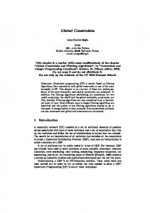
Algorithm 1 constructs the following formulae: x(A, 1, 1) ≡ x(a, 1, 1) x(A, 2, 1) ≡ x(a, 2, 1) x(B, 3, 1) ≡ x(b, 3, 1) x(A, 1, 2) ≡ x(a, 1, 1) ∧ x(A, 2, 1) x(B, 2, 2) ≡ x(b, 2, 1) ∧ x(B, 3, 1) x(S, 1, 3) ≡ (x(A, 1, 1) ∧ x(B, 2, 2)) ∨ (x(A, 1, 2) ∧ x(B, 3, 1))
x(S, 1, 3) ≡ ∨ x(A, 1, 2) ≡ ∨
∧
∧
∧
∨ ≡ x(B, 2, 2) ∧
x(a, 1, 1)
x(a, 2, 1)
x(A, 1, 1)
x(A, 2, 1)
x(b, 2, 1)
x(b, 3, 1) x(B, 3, 1)
Fig. 1. DAG corresponding to the example grammar.
The formulae created by Algorithm 1 can be represented by a rooted DAG. Every leaf is labelled with a variable x(t, i, 1) where t is a terminal symbol and i is an integer between 1 and n. Every inner-node is either a conjunction or a disjunction. Formulae of the form x ≡ b are represented by a single leaf node with two labels: x and b. For formulae of the form x ≡ (a1 ∧ b1 ) ∨ . . . ∨ (ak ∧ bk ), we create k and-nodes with two children each, ai and bi . We label each and-node with the expression ai ∧ bi . The k and-nodes have the or-node labelled with x as common parent. Based on this DAG, we propose the following CNF decomposition. For every ornode x with children c1 , . . . , ck , we post the following constraint forcing at least one child to be true when the or-node x is true. ¬x ∨ ci ∨ . . . ∨ ck
(1)
For every and-node x with children c1 and c2 , we post the following constraints to enforce all children to be true whenever the and-node x is true. ¬x ∨ c1 ¬x ∨ c2
(2) (3)
For every node x, except the root x(S, 1, n), we post the following constraint on its ancestors a1 , . . . , ak , to force the node x to be true only if one of its ancestors is true. ¬x ∨ a1 ∨ . . . ∨ ak
(4)
We force the root node x(S, 1, n) to be true. Finally, for every position 1 ≤ i ≤ n, we force one and only one terminal to be true. _ x(t, i, 1) ∀ 1 ≤ i ≤ n (5) t
¬x(t, i, 1) ∨ ¬x(u, i, 1) ∀ i ∀ t 6= u
(6)
Note that constraints (4) are redundant as they are logically implied by the others. However, they are added to the encoding to ensure that unit propagation on the decomposition prunes all possible values. Example 3. Let w be the node x(b, 2, 1)∧x(B, 3, 1), y be the node x(A, 1, 2)∧x(B, 3, 1), and z be the node x(A, 1, 1) ∧ x(B, 2, 2) in the DAG of Figure 1. We show the CNF clauses constraining the variable y. Clause (1) applied to x(S, 1, 3) becomes ¬x(S, 1, 3) ∨ y ∨ z. This ensures that if x(S, 1, 3) is true, one of its children is also true. Clauses (2) and (3) applied to y become ¬y ∨ x(A, 1, 2) and ¬y ∨ x(B, 3, 1). If the and-node y is true, both of its children are also true. Clause (4) constrains the variable y in three different ways. When the clause is directly applied to y, it becomes ¬y∨x(S, 1, 3) forcing y to be true only if it produces x(S, 1, 3). Similarly, the node x(A, 1, 2) belongs to a parsing tree only if y is true. We therefore have ¬x(A, 1, 2) ∨ y. Finally, the node x(B, 3, 1) is true only if either of its parents y or w is true. We therefore have ¬x(B, 3, 1) ∨ w ∨ y. There are no other constraints on variable y.
4
Theoretical properties
We first prove that this decomposition of the global G RAMMAR constraint is correct. The correctness follows quite quickly from the proof of the correctness of the CYK parser, and is similar to the correctness proofs for the previous propagators for the G RAMMAR constraint [3, 2]. Theorem 1 The G RAMMAR constraint is satisfiable iff x(S, 1, n) can be true. Proof: Suppose the G RAMMAR constraint is satisfiable. There exists a parsing tree T proving that the sequence X1 , . . . , Xn belongs to the language. We first prove that for every node in the parsing tree, there is a corresponding variable created by Algorithm 1.
We then show that all these variables can be set to true. The first phase of the algorithm (line 1 to line 7) stores in V [i, j] every non-terminal that can produce the symbols for Xi to Xi+j−1 . The second phase of the algorithm (line 8 to line 24) creates a node x(A, i, j) for every terminal A that can produce the symbols for Xi to Xi+j−1 and participates to the production of the non-terminal S at the root of the parsing tree. The correctness of this statement follows from [3, 2]. Therefore, for every node in the parsing tree T , we have a corresponding variable x(X, i, j). We prove by induction on the depth of the parsing tree that every variable corresponding to a node in the parsing tree can be set to true. As a base case, the leaves of the parsing tree correspond to the nodes x(Xi , i, 1) in the DAG that we set to true. The other leaves of the DAG are set to false. The clauses (5) and (6) are satisfied since there is one and only one leaf set to true at each position. Let A be a node in the parsing tree with children B and C where A generates a sequence of length j at position i and B generates a sequence of length k. Consequently, there exists a production A → BC ∈ G, a variable x(A, i, j), a variable x(B, i, k), and a variable x(C, i + k, j − k). On line 18, Algorithm 1 has made the node x(A, i, j) the parent of the pair x(B, i, k) ∧ x(C, i + k, j − k) since the production A → BC and both nodes x(B, i, k) and x(C, i + k, j − k) exist. By our induction hypothesis, we assume that the variables x(B, i, k) and x(C, i + k, j − k) are true. The and-node can be set to true while satisfying the clauses (2) and (3). Since the and-node is true, we can set the variable x(A, i, j) to true and satisfy clause (1). Finally, the clause (4) is satisfied for the variables x(B, i, k) and x(C, i + k, j − k) and the and-node. When applying the induction step to all nodes in the parsing tree in post-order, we obtain that the root node x(S, 1, n) can be set to true. Suppose there exists a solution to the CNF clauses where x(S, 1, n) is true. Clause 1 guarantees that at least one child is also true. This child is an and-node with two children that are also true thanks to the clauses (2) and (3). We continue this reasoning until reaching the leaf nodes. All the visited nodes form a parsing tree whose leaves, when listed from left to right, are a sequence satisfying the G RAMMAR constraint. Notice that the constraint (4) was not used in the second part of proof of Theorem 1. This constraint is not necessary to detect the satisfiability of the constraint. Constraint (4) is in fact redundant. It is however essential to prove our next result. We show that the decomposition of the G RAMMAR constraint does not hinder propagation. This is less immediate than the previous result. In particular, we find it surprising that unit propagation alone is enough to achieve GAC here. This does not follow directly from the completeness proofs for previous GAC propagators [3, 2]. Indeed, we had to add redundant constraints to the decomposition to give this property. Theorem 2 Unit propagation on the CNF clauses achieves GAC on the G RAMMAR constraint. Proof: We assume that all CNF clauses are consistent. The constraint (4) guarantees that every node that can be true has an ancestor that can also be true. By successively applying the argument from a leaf node x, we obtain a path connecting the leaf x to the root node x(S, 1, n) such that every variable on this path can be set to true. Let x(A, i, j) be a variable on the path. Let c1 , . . . , cn be the child variables of x(A, i, j) in
the DAG. From the constraint (1), we conclude that there exists at least one and-node among the children that can be true. Let ci be one such child that has b1 and b2 as children. The constraints (2) and (3) guarantee that both children can be true. We repeat this argument until reaching the leaves. Every node thus explored form a parsing tree whose leaves are a support for the variable x. Therefore, one can build a support for every node in the DAG that can be set to true. The constraint (5) ensures that if a character belongs to all supports, its corresponding leaf is fixed to true. Finally, the constraint (6) ensures that a character fixed to true removes all supports for the other characters at the same position. Finally, we show that we can propagate this decomposition efficiently. The run-time complexity of Algorithm 1 is the same as that of the CYK parser, i.e. Θ(n3 |G|) where |G| is the size of the grammar. Theorem 3 The running time complexity of Algorithm 1 is O(|G|n3 ) where n is the length of the sequence and |G| is the number of productions in the grammar. Proof: Line 2 iterates n times over the O(|G|) productions resulting in a time complexity of O(|G|n). The set V [i, j] created on line 7 tests all combinations of productions and integers between 1 and j for a total number of O(|G|n) tests. Since there are O(n2 ) sets V [i, j], the complexity sums up to O(|G|n3 ). The running time of the for loop on line 12 is dominated by the computation on line 15. Let Z be the set of non-terminals in the grammar. Let f (A) be the number P of productions in the grammar G whose left hand side is the non-terminal A. We have A∈Z f (A) = |G|. Line 15 takes O(nf (A)) time to execute as we test for each production that generates A and every integer k. The cumulative time spent on this line is therefore given by the following expression. n n−j+1 n X n X X X X X O( nf (A)) = O(n f (A)) j=2
i=1
A∈Z
(7)
j=1 i=1 A∈Z
= O(|G|n3 )
(8)
The running time of Algorithm 1 is thus O(|G|n)+O(|G|n3 )+O(|G|n3 ) = O(|G|n3 ). The size of the graph and the number of CNF clauses are bounded by the number of and-nodes in the DAG which is O(n3 |G|). Notice that whilst Algorithm 1 performs Θ(n3 |G|) tests on line 7, not all these tests add a non-terminal to the set V [i, j]. Moreover, not all the non-terminals in V [i, j] lead to the creation of a node on lines 15 to 18. We are now ready to analyse the running time complexity of maintaining GAC on the decomposition. We assume that the solver wakes up a constraint only when a variable in its scope is fixed to a specific value. For a CNF clause of arity k, this event occurs at most k times down the branch of the search tree. We have no assumptions regarding in which order the constraints are awaken. However, we assume that the propagator of a CNF clause of arity k maintains GAC in O(k) time down a branch of the search Wk tree. This assumption can be satisfied by encoding the k-ary CNF clause i=1 xi using the following clauses: x1 ∨ y2 , ¬yi ∨ xi ∨ yi+1 for 1 < i < k, and ¬yk ∨ xk . Since each of the k clauses is awaken at most three times down a branch of the search tree
and each propagation takes constant time, propagating the original CNF clause requires O(k) time down a branch of the search tree. Notice that other implementations of the CNF clause propagator might be more efficient in practice. See [13] for instance for an implementation using watched literals. Theorem 4 Amortised over a branch of the search tree of length k, we can enforce GAC k times on the G RAMMAR constraint using the decomposition in O(n3 |G|) time. Proof: We assume that propagating a CNF clause of arity k takes O(k) time down a branch of the search tree. We conclude that the propagation time, down a branch of the search tree, is proportional to the number of literals in the CNF clauses. Since the graph inducing the CNF clauses is of size O(n3 |G|), the number of literals in the CNF clauses is also O(n3 |G|). Consequently, we obtain a running time complexity of O(n3 |G|) down a branch of the search tree. This improves upon the Θ(n3 |G|) time complexity of the monolithic propagators for the G RAMMAR constraint given in [2, 3]. We note that our decomposition is the first incremental propagator proposed in the literature.
5
Regular languages
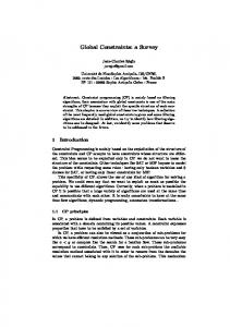
In some cases, we can specify problem constraints using a simple grammar. For instance, we often only need a regular language [1]. Regular languages are strictly contained within context-free languages. They can be specified with productions of the form of A → aB or A → a. We show that for regular languages, Algorithm 1 creates a smaller DAG, resulting in faster propagation. Theorem 5 Unit propagation on the CNF decomposition enforces GAC on the R EGULAR constraint in O(n|G|) time. Proof: If all productions are of the form of A → aB or A → a, a node x(A, i, j) can belong to a parsing tree only if i = n − j + 1. The size of the graph is therefore bounded by O(n|G|) and-nodes which limits the number of literals in the CNF clauses to O(n|G|). Using the same assumption and argument as Theorem 4, we conclude that propagating the CNF-clauses down a branch of the search tree takes O(n|G|) time. The running time complexity for pruning regular languages using this decomposition matches the complexity of the propagator for the R EGULAR constraint based on dynamic programming [1]. In fact, the clauses constructed by Algorithm 1 are essentially the hidden variable encoding of the ternary decomposition of the R EGULAR constraint given in [2]. Example 4. The language an bm used in Example 1 can be recognized by the automaton of Figure 2. This automaton can be translated to a regular grammar as follows. S → aA
A → aA | bB | b
B → bB | b
Algorithm 1 constructs the graph depicted in Figure 3 over a sequence of three variables. From this graph, we construct clauses representing the Boolean formulae:
a
S
a
b b
A
B
Fig. 2. Automaton recognizing the language an bm for n, m ≥ 1.
x(S, 1, 3) ≡ ∨ ∧ ∨ ≡ x(A, 2, 2) ∧
x(a, 1, 1)
x(a, 2, 1)
x(b, 2, 1)
∧
x(b, 3, 1) x(A, 3, 1) x(B, 3, 1)
Fig. 3. DAG corresponding to the regular grammar of Example 4.
x(a, 1, 1) ∧ (x(a, 2, 1) ∧ x(b, 3, 1)) ∨ (x(b, 2, 1) ∧ x(b, 3, 1)) This gives constraints logically equivalent to: X1 = a, (X2 = a ∧ X3 = b) ∨ (X2 = b ∧ X3 = b)
6
Conditional productions
We have also found it useful in practice to go slightly outside context-free grammars. These extensions permit us to specify in a simple manner that, for instance, a work day must have a span of between 6 to 8 hours, or that a certain activity can only be executed after 2pm. To specify such conditions, we make productions in the grammar conditional on Boolean functions of the relevant indices. This can be quickly incorporated into our decomposition. We attach the Boolean functions fA (i, j), fB (i, j), and fC (i, j) to every
production A → BC ∈ G. These functions restrict where the production can be applied in a sequence. For instance, the non-terminal A can only be produced by the production A → BC if A generates a sub-string of length j starting at position i where fA (i, j) is true. Similarly, the production can be applied only if B generates a sub-string of length j starting at position i where fB (i, j) is true. To support these constrained productions, we change line 7 in Algorithm 1 with the following one. V [i, j] ← {A | A → BC ∈ G, k ∈ [1, j), B ∈ V [i, k], C ∈ V [i + k, j − k], fA (i, j) ∧ fB (i, k) ∧ fC (i + k, j − k)} We also replace line 15 with the following one. D ← {hx(B, i, k), x(C, i + k, j − k)i | k ∈ [1, j), A → BC ∈ G, B ∈ V [i, k], C ∈ V [i + k, j − k], fA (i, j) ∧ fB (i, k) ∧ fC (i + k, j − k))} Productions of the form A → a only require a function fA (i) as they necessarily produce sequences of length one. Moreover, the production of a terminal can be controlled by removing the terminal from the domain of the variables Xi . We therefore replace line 2 with the following one. V [i, 1] ← {A | A → a ∈ G, a ∈ dom(Xi ), fA (i)} ∪ dom(Xi ) We also replace line 23 with the following one. Y ← Y ∪ {x(A, i, 1) ≡ x(a, i, 1) | A → a ∈ G, x(A, i, 1) ∈ N, a ∈ dom(Xi ), fA (i)}
7
Experimental results
To test the practical utility of this decomposition of the G RAMMAR constraint, we ran some experiments using the shift-scheduling benchmark introduced in [4]. The schedule of an employee in a company is subject to the following rules. An employee either works on an activity ai , has a break (b), has lunch (l), or rests (r). When working on an activity, the employee works on that activity for a minimum of one hour. An employee can change activities after a break or a lunch. A break is fifteen minutes long and a lunch is one hour long. Lunches and breaks are scheduled between periods of work. A part-time employee works at least three hours but less than six hours a day and has one break. A full-time employee works between six and eight hours a day and have a break, a lunch, and a break in that order. Employees rest at the beginning and the end of the day. At some time of the day, the business is closed and employees must either rest, break, or have lunch. We divide a day into 96 time slots of 15 minutes. During time slot t, at least d(t, ai ) employees must be assigned to activity ai . Our goal is to minimize first the number of employees and then the number of hours worked. We model the schedule of an employee with a sequence of 96 characters (one per time slot) that must be accepted by the following grammar G. R → rR | r W → Ai S → RP R | RF R
L → lL | l P → W bW
Ai → ai Ai | ai F → P LP
We add some restrictions on some productions. For W → Ai , we have fW (i, j) ≡ j ≥ 4 since an employee works on an activity for at least one continuous hour. In F → P LP , we have fL (i, j) ≡ (j = 4) since a lunch is one hour long. In S → RP R, we have fP (i, j) ≡ 13 ≤ j ≤ 24 since a part-time employee works at least three hours and at most six hours plus a fifteen minute break. In S → RF R, we have fF (i, j) ≡ 30 ≤ j ≤ 38 which represents between six and eight hours of work plus an hour and a half of idle time for the lunch and the breaks. Finally, the productions Ak → ak Ak | ak are constrained with fAk (i, j) ≡ open(i) where open(t) returns true if t is within business hours. When solving the problem with m employees, the model consists of m sequences S1 , . . . , Sm subject to this G RAMMAR constraint. The th 0/1 variable Px(j, t, c) is set to 1 if the t character of sequence Sj is c. We post the constraint j x(j, t, ai ) ≥ d(t, ai ) in order to satisfy the demand for each activity ai at time t. To break symmetry, we force the sequences to be in lexicographical order. We implemented a program that takes as input a benchmark instance and the grammar G and prepares the input for the MiniSat+ solver [5]. MiniSat+ is a pseudo-Boolean solver that allows constraints of the form x1 + . . . + xn ≥ k where xi is a Boolean variable. Such inequality constraints are useful to make sure that the demand d(t, ai ) is satisfied. CNF clauses are encoded with linear equations where the sum of the literals in a clause must be equal to or greater than one. The negation of a variable x is expressed with 1 − x. We tested two CNF encodings of the G RAMMAR constraint: one encoding that includes the redundant clause (4) allowing unit propagation to achieve GAC as well as one encoding where the clauses (4) are omitted and GAC is not maintained. We also implemented a CP model in ILog Solver 6.2 using either this decomposition of the G RAMMAR constraint or the previous monolithic propagator for the G RAMMAR constraint based on the CYK parser [2, 3]. The model has a matrix of variables where each row corresponds to the schedule of an employee and is subject to a G RAMMAR constraint. Each column is subject to a global cardinality constraint (GCC) to ensure that the number of occurrences of an activity satisfies the demand. We added lexicographic constraints between the rows of the column to break symmetries. We used a static variable that was essential to the success of the experiment: we filled in the table from left to right, and assigned variables to the values r, b, l, a1 and a2 in that order. Our experiments used MiniSat+ on a Intel Dual Core 2.0 GHz with 1 Gb of RAM using Mac OS X 10.4.8 and ILog Solver on a AMD Dual Core Opteron 2.2 GHz with 4 Gb of RAM. The reader should be careful when comparing the times as the clock speeds of the computers are slightly different. MiniSat+ is halted after finding the optimal solution or when the search is suspended by a lack of memory. ILog solver was halted after one hour of computation as it never proved the optimality of a solution. Table 1 presents the results for 17 satisfiable instances of the benchmark involving one or two activities. The CP model performed very well at finding a good solution. Many solutions were returned after a few hundreds of backtracks. However, no solutions were proved optimal after one hour of computation. Notice that the decomposition performs significantly better than the monolithic propagator as it explores many more backtracks within the same period of time. The decomposition therefore explores a larger portion of the search tree. For some instances, it finds some satisfiable solutions within one hour whereas the monolithic propagator does not.
|A| # m
GAC SAT SAT Mono Decomp sol time bt opt sol time bt opt sol bt sol bt √ √ 1 2 4 26.0 2666 507215 26.0 1998 443546 26.75 28072 26.25 625683 1 3 6 37.25 1128199 36.75 1953562 37.0 34788 37.0 4771577 √ √ 1 4 6 38.0 256 84999 38.0 287 91151 - 15539 38.0 56488 √ √ 1 5 5 24.0 153 67376 24.0 60 40008 24.0 40163 24.0 7914413 √ √ 1 6 6 33.0 98 48638 33.0 70 40361 - 11537 33.0 33405 1 7 8 49.5 236066 49.5 682715 49.0 27635 49.0 2663721 √ √ 1 8 3 20.5 80 36348 20.5 44 25502 21.0 24343 20.5 635589 1 10 9 54.0 202699 54.25 507749 - 9365 - 519446 √ 2 1 5 25.0 453 146234 25.0 301 103918 25.0 1180 25.0 3828461 2 2 10 58.75 313644 59.0 151076 58.0 14887 58.0 2116602 2 3 6 38.25 236850 38.25 214203 41.0 1419 41.0 214201 2 4 11 71.25 230777 69.75 239519 - 9983 - 774942 √ √ 2 5 4 23.75 2945 644496 23.75 1876 522780 26.5 25573 26.25 117105 √ 2 6 5 26.75 4831 777572 27.25 2162816 26.75 10681 26.75 1054531 244837 31.75 391858 32.0 218 31.5 3771831 2 8 5 31.5 √ √ 2 9 3 19.0 2283 701474 19.0 1227 481395 19.25 20473 19.0 45516 2 10 8 55.0 372870 55.0 333520 - 9968 - 909857 Table 1. Benchmark problems solved by MiniSat+. GAC SAT: results from MiniSat+ with all CNF clauses; SAT: results from MiniSat+ with all CNF clauses but clause (4); Mono: results from a CP solver using the monolithic propagator; Decomp: results from a CP solver using the decomposition; |A|: number of activities; #: problem number; m: number of employees; sol: number of worked hours (boldfonted if best solution found amongst the different methods); time (s): CPU time in seconds to find and prove the optimality of a solution. Times are omitted when the search is suspended by a lack of memory; bt: number of backtracks (boldfonted if least backtracks amongst methods that prove optimality); opt: solution was proved optimal. ILog solver did not prove any problems optimal within one hour of computation.
The MiniSat+ solver returned a feasible solution for all instances regardless of the encoding. For 8 instances, the solver also proved optimality of the solutions. However, the two encodings we used did not prove optimality for the same instances. The main weakness of the MiniSat+ solver was its memory consumption as 9 times out of 17, the search was stopped by the lack of memory. Notice that the encoding that omits clauses of the form (4) is often faster than the encoding achieving GAC. We conjecture that, in this case, MiniSat is finding itself the redundant constraints using no-good learning. Even though Algorithm 1 can produce a graph with up to O(n3 |G|) nodes, we noticed that in practice many nodes are never created. The size of the resulting DAG is much smaller in practice than the theoretical bound of O(n3 |G|). For instance, the grammar G for problems with one activity can be written in Chomsky normal form in 3 15 productions. The upper bound on the number of and-nodes in the DAG is 15 962 = 6635520 nodes whilst there were 71796 nodes on average with these instances. We also tried modelled the schedule of an employee using an automaton. Due to the constraints on the number of hours a full-time and a part-time employee must work, many states in the automaton needed to be duplicated resulting in an automaton with several thousands of states. Moreover, patterns such as those produced by the non-
terminals P and W cannot be reused in an automaton without further duplicating states. The DAG based on the regular language ended up much larger than the one produced by the context-free grammar.
8
Related work
Vempaty introduced the idea of representing the solutions of a CSP by a deterministic finite automaton [6]. Such automaton can be used to answer questions about satisfiability, validity and equivalence. Amilhastre generalized these ideas to non-deterministic automata, and proposed heuristics to minimize the size of the automata [7]. This approach was then applied to configuration problems [8]. Boigelot and Wolper developed decision procedures for arithmetic constraints based on automata [9]. Pesant introduced the R EGULAR constraint and gave a complete propagation algorithm based on dynamic programming [1]. Coincidently Beldiceanu, Carlsson and Petit proposed specifying global constraints by means of finite automaton augmented with counters [10]. Propagators for such automaton are constructed automatically from the specification of the automaton by means of a decomposition into simpler constraints. Quimper and Walsh proposed a closely related decomposition of the R EGULAR constraint and showed that it was effective and efficient in practice [2]. Demassay et al. [4] used a column generation technique to solve a shift scheduling problem. The columns are generated with a CP solver using the C OST-R EGULAR constraint, a variation of the R EGULAR constraint while the optimization process is driven by the simplex method. Cˆot´e et al. [11] encoded the R EGULAR constraint into a MIP and efficiently solved some instances of the shift scheduling problem using the same automaton as Demassay et al. This encoding takes the modelling of constraints using formal languages beyond the scope of constraint programming. One of our contributions is to continue this theme by taking constraints specified using formal languages into the domain of SAT solvers. Quimper and Walsh proposed the G RAMMAR constraint and gave two different propagators, one based on the CYK and the other on the Earley parser [2]. Coincidently, Sellmann proposed the G RAMMAR constraint and gave a propagator based on the CYK parser [3]. Finally Golden and Pang proposed the use of string variables which are specified using regular expressions or finite automata and show how to propagate matching, containment, cardinality and other constraints on such string variables [12].
9
Conclusion
We have studied the global G RAMMAR constraint. This restricts a sequence of variables to belong to a context-free language. Such a constraint is useful for a wide range of problems in scheduling, rostering and related domains. Based on an AND/OR decomposition, we showed how the G RAMMAR constraint can be converted into clauses in conjunctive normal form. This decomposition does not hinder propagation since unit propagation on the decomposition achieves GAC on the original G RAMMAR constraint. Using this decomposition, we can enforce GAC on the G RAMMAR constraint in O(n3 ) time. By using the decomposition, we also improve upon existing propagators by being incremental. On specialized languages, running time can be even better. In particular,
on regular languages we require just O(n|δ|) time where |δ| is the size of the transition table of the automaton recognizing the language. Experiments on a shift scheduling problem with a state of the art SAT solver demonstrated that we can solve problems this way that defeat existing constraint solvers. The decomposition of global constraints opens up a number of possibilities which we are only starting to explore. For example, it may make it easier to construct no-goods, as well as cost measures for over-constrained problems. Finally, a decomposition may make it easier to construct constraint based branching heuristics.
Acknowledgements The second author is funded by DCITA and the ARC through Backing Australia’s Ability and the ICT Centre of Excellence program. We would like to thank Louis-Martin Rousseau for useful comments and for providing the benchmark.
References 1. Pesant, G.: A regular language membership constraint for finite sequences of variables. In: 10th Int. Conf. on Principles and Practice of Constraint Programming (CP2004), LNCS 3258 (2004) 482–295 2. Quimper, C.-G., Walsh, T.: Global grammar constraints. In: 12th Int. Conf. on Principles and Practices of Constraint Programming (CP-2006), LNCS 4204 (2006) 3. Sellmann, M.: The theory of grammar constraints. In: 12th Int. Conf. on Principles and Practice of Constraint Programming (CP2006), LNCS 4204 (2006) 530–544 4. Demassey, S., Pesant, G., Rousseau, L.: A cost-regular based hybrid column generation approach. Constraints 11 (2006) 315–333 5. E´en, N., S¨orensso, N.: Translating pseudo-Boolean constraints into SAT. Journal on Satisfiability, Boolean Modelling and Computation 2 (2006) 1–26 6. Vempaty, N.R.: Solving constraint satisfaction problems using finite state automata. In: 10th National Conf. on AI, AAAI (1992) 453–458 7. Amilhastre, J.: Representation par automate d’ensemble de solutions de probl`emes de satsifaction de contraintes. PhD thesis, Universite Montpellier II / CNRS, LIRMM (1999) 8. Amilhastre, J., Fargier, H., Marquis, P.: Consistency restoration and explanations in dynamic CSPs - application to configuration. Artificial Intelligence 135 (2002) 199–234 9. Boigelot, B., Wolper, P.: Representing arithmetic constraints with finite automata: An overview. In: Int. Conf. on Logic Programming (ICLP 2002), LNCS 2470 (2002) 1–19 10. Beldiceanu, N., Carlsson, M., Petit, T.: Deriving filtering algorithms from constraint checkers. In: 10th Int. Conf. on Principles and Practice of Constraint Programming (CP2004), LNCS 3258 (2004) 107–122 11. Cˆot´e, M.C., Gendron, B., Rousseau, L.M.: The regular constraint for integer programming modeling. In: 4th Int. Conf. on Integration of AI and OR Techniques in Constraint Programming (CPAIOR 07). (2007) 29–43 12. Golden, K., Pang, W.: Constraint reasoning over strings. In: 9th Int. Conf. on Principles and Practice of Constraint Programming (CP2003), LNCS 2833 (2003) 377–391 13. Moskewicz, M., Madigan, C., Zhao, Y., Zhang, L., and Malik, S.: CHAFF: engineering an efficient SAT solver. In Proc. of the 38th Design Automation Conf. (DAC’01). (2001) 530–535