viewed as decomposition methods. 3 Dynamic Decomposition Methods. One of the advantages of the cutting plane method over traditional decomposition ...
Decomposition and Dynamic Cut Generation in Integer Programming: Theory and Algorithms T.K. Ralphs∗
M.V. Galati†
Revised November 23, 2003
Abstract Decomposition algorithms such as Lagrangian relaxation and Dantzig-Wolfe decomposition are well-known methods that can be used to compute bounds for integer programming problems. We discuss a framework for integrating dynamic cut generation with traditional decomposition methods in order to obtain improved bounds and present a new paradigm for separation called decompose and cut. The methods we present take advantage of the fact that separation of a vector with known structure is often much easier than separation of an arbitrary one.
1
Introduction
In this paper, we discuss new methods for computing bounds on the value of an optimal solution to a large-scale mixed-integer linear program (MILP)1 that integrate dynamic cut generation with traditional decomposition techniques. Computing bounds is an essential element of the branch and bound algorithm, which is the most effective and most commonly used method for solving such mathematical programs. Bounds are typically computed by solving a bounding subproblem, which is either a relaxation or a dual of the original problem. The most commonly used bounding subproblem is the linear programming (LP) relaxation. The LP relaxation is often too weak to be effective in solving difficult MILPs, but it can be strengthened by adding dynamically generated valid inequalities to the relaxation. Alternatively, traditional decomposition techniques, such as DantzigWolfe decomposition [8] or Lagrangian relaxation [11, 7], can also be used to obtain improved bounds. In what follows, we show how to combine the two methods to obtain a new class of bounding procedures called dynamic decomposition methods. We also develop a new paradigm for performing separation using decomposition techniques. To simplify the exposition, we consider only pure integer linear programming problems (ILPs) with finite upper and lower bounds on all variables. The framework can easily be extended to more general settings. For the remainder of the paper, we consider an ILP instance whose feasible set is the integer vectors contained in the polyhedron Q = {x ∈ x} = min{c> x} = minn {c> x : Ax ≥ b} x∈F
x∈P
x∈
Z
(1)
for a given cost vector c ∈ Qn . A related problem is the separation problem for P. Given x ∈ Rn , the problem of separating x from P is that of deciding whether x ∈ P and if not, determining a ∈ Rn and β ∈ R such that a> y ≥ β ∀y ∈ P but a> x < β. A pair (a, β) ∈ Rn+1 such that a> y ≥ β ∀y ∈ P is a valid inequality 2 for P and is said to be violated by x ∈ Rn if a> x < β. In [14], it was shown that the separation problem for P is polynomially equivalent to the optimization problem for P. To apply the principle of decomposition, we consider the relaxation of (1) defined by min {c> x} = min0 {c> x} = minn {c> x : A0 x ≥ b0 },
x∈F 0
(2)
Z
x∈
x∈P
0
0
where F ⊂ F 0 = {x ∈ Zn : A0 x ≥ b0 } for some A0 ∈ Qm ×n , b0 ∈ Qm . As usual, we assume that there exist effective3 algorithms both for optimizing over and separating from P 0 . Along with P 0 00 00 is associated a set of side constraints. Let [A00 , b00 ] ∈ Qm ×n be a set of additional inequalities needed to describe F, i.e., [A00 , b00 ] is such that F = {x ∈ Zn : A0 x ≥ b0 , A00 x ≥ b00 }. We denote by Q0 the polyhedron described by the inequalities [A0 , b0 ] and by Q00 the polyhedron described by the inequalities [A00 , b00 ]. Hence, the initial LP relaxation is the linear program defined by Q = Q0 ∩ Q00 , and the LP bound is given by zLP = min{c> x} = minn {c> x : A0 x ≥ b0 , A00 x ≥ b00 }. x∈Q
x∈
R
(3)
Note that this is slightly more general than the traditional framework, in which [A0 , b0 ] and [A00 , b00 ] are a partition of the rows of [A, b] into a set of “nice constraints” and a set of “complicating constraints.”
2
Traditional Decomposition Methods
The goal of the decomposition approach is to improve on the bound obtained using the initial LP relaxation (zLP ) by taking advantage of our ability to optimize over and/or separate from P 0 . In this section, we briefly review the classical bounding methods that take this approach. 00
Lagrangian Relaxation. For a given vector of dual multipliers u ∈ Rm + , the Lagrangian relaxation of (1) is given by zLR (u) = min0 {(c> − u> A00 )s + u> b00 } (4) s∈F
It is easily shown that zLR (u) is a lower bound on zIP for any u ≥ 0. The problem zLD = max00 {zLR (u)}
Rm+
(5)
u∈
of maximizing this bound over all choices of dual multipliers is a dual to (1) called the Lagrangian dual (LD) and also provides a lower bound zLD , which we call the LD bound. A vector of multipliers u ˆ that yield the largest bound are called optimal (dual) multipliers. 2
Note that we assume all inequalities are expressed in “≥” form. The term effective is not defined rigorously, but denotes an algorithm with a “reasonable” average-case running time. 3
2
The Lagrangian dual can either be solved using subgradient optimization or by rewriting it as the equivalent linear program zLD =
max
R Rm+ 00
{α + u> b00 : α ≤ (c> − u> A00 )s ∀s ∈ F 0 }.
(6)
α∈ ,u∈
In either case, most of the computational effort goes into evaluating zLR (u) for a given sequence of dual multipliers u. This is an optimization problem over P 0 and can be solved effectively by assumption. Both of these approaches are described in detail in [18]. Dantzig-Wolfe Decomposition. The approach of Dantzig-Wolfe decomposition is to reformulate (1) by implicitly requiring the solution to be a member of F 0 , while explicitly enforcing the inequalities [A00 , b00 ]. Relaxing the integrality constraints of this reformulation, we obtain the linear program X X X zDW = min 0 {c> ( sλs ) : A00 ( sλs ) ≥ b00 , λs = 1}, (7)
RF+
λ∈
s∈F 0
s∈F 0
s∈F 0
which we call a Dantzig-Wolfe LP (DWLP). Although the number of columns in this linear program is |F 0 |, it can be solved by dynamic column generation, where the column-generation subproblem is again an optimization problem over P 0 . For this reason, Dantzig-Wolfe is sometimes referred to generically as a column-generation method. Applying Dantzig-Wolfe decomposition within the context of branch and bound results in a method known as branch and price [5]. It is easy to verify that the DWLP is the dual of (6), which immediately shows that zDW = zLD (see [19] for a treatment of this fact). Hence, zDW is a valid lower bound on zIP that we call the DW bound. Note that the dual variables in the DWLP correspond to the dual multipliers from ˆ an optimal solution to the Section 2. Furthermore, if we combine the members of F 0 using λ, Dantzig-Wolfe LP, to obtain X ˆs, x ˆ= sλ (8) s∈F 0
then we see that zDW = c> x ˆ. Since x ˆ must lie within P 0 ⊆ Q0 and also within Q00 , this shows that zDW ≥ zLP . Cutting Plane Method. In the cutting plane method, which is described in more detail in Section 3, inequalities describing P 0 (i.e., the facet-defining inequalities) are generated dynamically by separating the solutions to a series of LP relaxations from P 0 . In this way, the initial LP relaxation is iteratively augmented to obtain the CP bound, zCP = min0 {c> x : A00 x ≥ b00 }. x∈P
(9)
Note that x ˆ, as defined in (8), is an optimal solution to this augmented linear program. Hence the CP bound is equal to both the DW bound and the LD bound. We refer to xˆ as an optimal fractional solution and the augmented linear program above as the cutting plane LP (CPLP). A Common Framework. Summarizing what we have seen so far, the following well-known result of Geoffrion [13] shows that the three approaches just described are simply three different algorithms for computing the same quantity. Theorem 1 zIP ≥ c> x ˆ = zLD = zDW = zCP ≥ zLP .
3
A graphical depiction of these bounds can be seen later in Figure 2. The close relationship of these three methods can be made even more explicit by viewing them in a common framework. In each of the three methods, we are given a polyhedron P, called the original polyhedron, over which we would like to optimize. In addition, we are given two polyhedra that contain P: an explicit polyhedron with a small description that can be represented explicitly (Q00 ) and an implicit polyhedron with a much larger description that must be represented implicitly (P 0 ). The conceptual difference between Dantzig-Wolfe decomposition, Lagrangian relaxation, and the cutting plane method is that both Dantzig-Wolfe decomposition and Lagrangian relaxation utilize an inner representation of P 0 , generated dynamically by solving the corresponding optimization problem, whereas the cutting plane method relies on an outer representation of P 0 , generated dynamically by solving the separation problem for P 0 . In this framework, most dynamic methods for solving ILPs, can be viewed as decomposition methods.
3
Dynamic Decomposition Methods
One of the advantages of the cutting plane method over traditional decomposition approaches is the option of adding heuristically generated valid inequalities to the CPLP to improve the bound. This can be interpreted as a dynamic tightening of either the explicit or the implicit polyhedron. We will focus on the former interpretation and propose several dynamic decomposition methods that use either a DWLP or an LD as the bounding subproblem. Note that it is also possible to develop analogs of these methods based on the latter interpretation—the development is similar. First consider the basic steps of the cutting plane method, assuming the problem at hand is feasible and bounded. To begin, we construct an initial LP relaxation and solve it. We then perform the separation step, attempting to generate inequalities valid for P but violated by the resulting solution. If successful, we add these inequalities to the LP relaxation, hoping to improve the bound. This procedure is iterated until no more violated inequalities are found. The most important step is that of separation, which results in a tightening of the explicit polyhedron and (hopefully) an improved bound. In principle, this procedure can be generalized by replacing the CPLP with either a DWLP or an LD as the bounding subproblem. We generically call the resulting method the dynamic decomposition method, The steps are generalized as shown in Figure 1. Again, the important step is Step 3, generating a set of improving inequalities, i.e., inequalities valid for P that when added to the description of the explicit polyhedron result in an increase in the computed bound. Aside from Step 3, the method is straightforward. Steps 1 and 2 are performed as in a traditional decomposition framework. Step 4 is accomplished by simply adding the newly generated inequalities to the list [A00 , b00 ] and reforming the appropriate bounding subproblem. The most important question to be answered is exactly how the constraint generation step (Step 3), which is the crux of the method, should be accomplished. In the cutting plane method, techniques for generating valid inequalities are well-studied, but there is no easily verifiable sufficient condition for an inequality to be improving. Violation of xˆ is a necessary condition for an inequality to be improving, and hence such an inequality is likely to be effective. However, unless the inequality separates the entire optimal face F to the CPLP, it will not be improving. Because we want to refer to these well-known results later, we state them formally as theorem and corollary without proof. See [23] for a thorough treatment of the theory of linear programming that leads to this result. Theorem 2 Let F be the face of optimal solutions to the CPLP. Then (a, β) ∈ Rn+1 is an improving inequality if and only if a> y < β for all y ∈ F .
4
Dynamic Decomposition Method 1. Construct the initial bounding subproblem P0 and set i ← 0. zCP = minx∈P 0 {c> x : A00 x ≥ b00 } zLR = maxu∈Rn+ minx∈P 0 {(c> − u> A00 )x + u> b00 } P P P zDW = minλ∈RF 0 {c> ( s∈F 0 sλs ) : A00 ( s∈F 0 sλs ) ≥ b00 , s∈F 0 λs = 1} +
2. Solve Pi to obtain a valid lower bound z i . 3. Attempt to generate a set of improving inequalities [Di , di ] valid for P. 4. If valid inequalities were¤ found in Step 3, form the bounding subproblem Pi+1 by £ 00 b00 setting [A00 , b00 ] ← A . Then, set i ← i + 1 and go to Step 2. Di di 5. If no valid inequalities were found in Step 3, then output z i . Figure 1: Basic outline of the dynamic decomposition method Corollary 1 If (a, β) ∈ Rn+1 is an improving inequality and x ˆ is an optimal solution to the CPLP, then a> x ˆ < β. In the next two sections, we discuss how improving inequalities can be generated when the bounding subproblem is either a DWLP or an LD. Then we return to the cutting plane method to discuss how decomposition can be used directly to improve our ability to solve the separation problem. Price and Cut. We first consider using a DWLP as the bounding subproblem in the procedure of Figure 1. We call this general approach price and cut. When employed in a branch and bound framework, the overall technique is called branch, price, and cut and has been studied by a number of authors [25, 16, 4, 24]. Simultaneous generation of columns4 and valid inequalities is difficult in general because the addition of valid inequalities tends to destroy the structure of the columngeneration subproblem (for a discussion of this, see [24]). Having solved the DWLP, however, we can easily recover an optimal solution to the CPLP using (8) and try to generate improving inequalities using traditional separation methods. The generation of those valid inequalities takes place in the original space and does not destroy the structure of the column-generation subproblem. Hence, the approach enables dynamic generation of valid inequalities while still retaining the bound improvement and other advantages yielded by a Dantzig-Wolfe decomposition. Note that the same bound improvement obtained in price and cut could be realized in the cutting plane method by adding the generated inequalities directly to the CPLP. Despite the apparent symmetry, there is one fundamental difference between the cutting plane method and price and cut. An optimal solution to the DWLP, which we shall henceforth refer to as an optimal decomposition, provides a decomposition of x ˆ from (8) into a convex combination of members of F 0 . In particular, the weight on each member of F 0 in the combination is given by the optimal decomposition. We refer to elements of F 0 that have a positive weight in this combination as members of the decomposition. The following theorem shows how the decomposition can be used 4
To be more precise, we should use the term variables here since “column generation” implies a fixed number of rows.
5
to derive an alternative necessary condition for an inequality to be improving. A formal proof can be found in [21]. Theorem 3 If (a, β) ∈ R(n+1) is an improving inequality, then there must exist an s ∈ F 0 with ˆ s > 0 such that a> s < β. λ In other words, an inequality can be improving only if it is violated by at least one member of the decomposition. This follows easily from the fact that the degree of violation of xˆ is a convex combination of the degrees of violation of each member of the decomposition. The importance of this result is that in some cases, it is much easier to separate members of F 0 from P than to separate arbitrary real vectors. In fact, it is easy to find polyhedra for which the problem of separating an arbitrary real vector is difficult, but the problem of separating a solution to a given combinatorial relaxation is easy. Some examples are discussed in Section 4. This leads to a new separation technique that can be embedded within price and cut. The idea is to replace direct separation of the fractional point (which may be difficult) with separation of members of the decomposition, which act as surrogates. Given a decomposition, the efficiency of this procedure depends both on the cardinality of the decomposition (which must be less than or equal to dim(P) + 1) and the time required to separate members of P 0 from P. Note that there are several potential pitfalls in implementing such a procedure. The biggest of these is that the set of inequalities violated by a member of the decomposition might be extremely large and it cannot easily be determined which of these inequalities will be improving. Generating the inequality most violated by x ˆ from the decomposition using this procedure is in fact a multi-criteria optimization problem, which may also be difficult. However, as a heuristic technique that allows a set of potentially violated inequalities to be generated quickly, this procedure shows great promise. Before moving on, we would like to draw some further connections between price and cut and the traditional cutting plane method that shed further light on the technique we have proposed. Solving the DWLP generally results in an optimal fractional solution that is contained in a proper face of P 0 . In fact, we can characterize precisely the face of P 0 in which x ˆ must be contained. Consider the set S = {s ∈ F 0 : (c> − u ˆ> A00 )s = (c> − u ˆ> A00 )ˆ s}, (10) where sˆ is some member of the decomposition (and hence corresponds to a basic variable in an optimal solution to the DWLP). The following theorem tells us that the set S must contain all members of the decomposition. The proof can be found in [21]. ˆ s > 0} ⊆ S. Theorem 4 {s ∈ F 0 : λ In fact, we can show something stronger—that the set S is comprised exactly of those members of F 0 corresponding to columns of the DWLP with reduced cost zero. This fact has important implications in the next section, where we use it to draw connections to another dynamic decomposition method. The following result follows from Theorem 4. The proof can be found in [21]. Theorem 5 conv(S) is a face of P 0 and contains x ˆ. An important consequence of this result is contained in the following corollary, which states that the face of optimal solutions to the cutting plane LP is contained in conv(S) ∩ Q00 . Corollary 2 If F is the face of optimal solutions to the CPLP, then F ⊆ conv(S) ∩ Q00 . 6
c> = c> − u ˆ > A00
s ˆ0
s ˆ1
c> − u ˆ > A00
s ˆ1
c>
xLP = x ˆ
P0
x ˆ
xLP
c>
s ˆ1
x ˆ
xLP
s ˆ0
s ˆ0
P0
00
Q
P0
Q00
Q00
Q0
s ˆ2
Q0
P 0 ∩ Q00 = conv(S) ∩ Q00
Q0
conv(S) ∩ Q00 = F
(a)
P 0 ∩ Q00 ⊃ conv(S) ∩ Q00 ⊃ F
(b)
(c)
0
ˆs > 0 s∈F :λ
conv(S)
Figure 2: Illustration of bounds for different cost vectors
Hence, the convex hull of the decomposition is a subset of conv(S) that contains x ˆ and can be thought of as a surrogate for the face of optimal solutions to the CPLP. Combining this corollary with Theorem 2, we conclude that separation of S from P is a sufficient condition for an inequality to be improving. Although this sufficient condition is difficult to verify in practice, it does provide additional motivation for the method described in the preceding paragraph. As noted earlier, conv(S) is typically a proper face of P 0 . It is possible, however, for x ˆ to be an inner point of P 0 . In this case, illustrated graphically in Figure 2(a), zDW = zLP and DantzigWolfe decomposition does not improve the bound. All columns of the DWLP have reduced cost zero and any extremal member of F 0 could be made a member of the decomposition. Hence, the effectiveness of the procedure is reduced and the chosen relaxation may be too weak. A necessary condition for an optimal fractional solution to be an inner point of P 0 is that the dual value of the convexity constraint in an optimal solution to the DWLP be zero. If this condition arises, then caution should be observed. This result is further examined in the next section. A second case of potential interest is when F = conv(S) ∩ Q00 , illustrated graphically in Figure 2(b). This condition can be detected by examining the objective function values of the members of the decomposition. If they are all equal, then any member of the decomposition that is contained in Q00 (if one exists) must be optimal for the original ILP, since it is feasible and has objective function value equal to zLP . In this case, all constraints of the DWLP other than the convexity constraint must have dual value zero, since removing them does not change the optimal solution value. The more typical case, in which F is a proper subset of conv(S) ∩ Q00 , is shown in Figure 2(c). Relax and Cut. We now move on to discuss the dynamic generation of valid inequalities when the bounding subproblem is an LD, a method known as relax and cut. When employed in a branch and bound framework, the overall method is called branch, relax, and cut and has also been studied previously by several authors (see [17] for a survey). Solving the LD as the linear program (6) is equivalent to solving the DWLP, so the methods just discussed apply directly without modification. We assume from here on that the LD is solved in the form (5), using subgradient optimization. 7
Suppose we have solved the LD to obtain u ˆ, a vector of optimal multipliers for the LD and P ˆ ˆ sˆ = argmin zLR (ˆ u). As before, let λ be an optimal decomposition and x ˆ = s∈F 0 sλs be an optimal fractional solution. The main consequence of using subgradient optimization to solve the LD is that we do not obtain the primal solution information available to us with both the cutting plane method and price and cut. This means there is no way of constructing an optimal fractional solution or verifying the condition of Corollary 1. We can, however, attempt to separate the solution to the Lagrangian relaxation (4), which is a member of F 0 , from P. Note that again, we are taking advantage of our ability to separate members of F 0 from P effectively. If successful, we immediately “dualize” this new constraint by adding it to [A00 , b00 ], as described in Section 3. This has the effect of introducing a new dual multiplier and slightly perturbing the objective function used to solve the Lagrangian relaxation. As with both the cutting plane and price and cut methods, the difficulty with relax and cut is that the valid inequalities generated by separating sˆ from P may not be improving, as Guignard first observed in [15]. As we have already noted, we cannot verify the condition of Corollary 1, which is the best available necessary condition for an inequality to be improving. To deepen our understanding of the potential effectiveness of the valid inequalities generated during relax and cut, we now further examine the relationship between sˆ and x ˆ. From the reformulation of the LD as the linear program (6), we can see that each constraint binding at an optimal solution corresponds to an alternative optimal solution to the Lagrangian subproblem with multipliers u ˆ. The binding constraints of (6) correspond to variables with reduced cost zero in the DWLP (7), so it follows immediately that the set of all alternative solutions to the Lagrangian subproblem with multipliers u ˆ is the set S from (10). Because x ˆ is both an optimal solution to the CPLP and is contained in conv(S), it also follows that c> x ˆ = (c> − u ˆ> A00 )ˆ x+u ˆ> b00 , In other words, the penalty term in the objective function of the Lagrangian subproblem (4) serves to rotate the original objective function so that it becomes parallel to the face conv(S), while constant term u ˆ> b00 ensures that x ˆ has the same cost with both the original and the Lagrangian objective function. This is shown in Figure 2(c). One conclusion that can be drawn from the above results is that the fundamental connection between relax and cut and price and cut is that solving the DWLP produces a set of alternative optimal solutions to the LD, at least one of which must be violated by a given improving inequality. This yields a verifiable necessary condition for a generated inequality to be improving. Relax and cut, on the other hand, produces only one member of this set, though possibly at a much lower computational cost. Even if improving inequalities exist, it is possible that none of them are violated by sˆ, especially if sˆ has a small weight in the optimal decomposition. As in price and cut, when x ˆ is an inner point of P 0 , the decomposition does not improve the bound and all members of 0 F are alternative optimal solutions to the Lagrangian subproblem dual multipliers uˆ. This situation is depicted in Figure 2(a). In this case, separating sˆ is unlikely to yield an improving inequality. Decompose and Cut. The use of an optimal decomposition to aid in separation is easy to extend to a traditional branch and cut framework using a technique originally proposed in [22], which we call decompose and cut. Suppose now that we are given an optimal fractional solution xˆ derived directly by solving the CPLP. Suppose again that given s ∈ F 0 , we can determine efficiently whether s ∈ F and if not, generate a valid inequality violated by s. By first decomposing x ˆ (i.e., expressing x ˆ as a convex combination of members of F 0 ) and then separating each member of the 8
decomposition from P, we obtain a separation methodology similar to that described in the section on price and cut. When employed within a branch and bound framework, we call the resulting method branch, decompose, and cut. The difficult step is finding the decomposition of x ˆ. This can be accomplished by solving a linear program X X max0 {0> λ : sλs = x ˆ, λs = 1}, (11)
R+F
λ∈
s∈F 0
s∈F 0
whose columns are the members of F 0 using a technique reminiscent of the column-generation scheme for solving the DWLP. This scheme can be seen as the “inverse” of the method described for price and cut, since it begins with the fractional solution xˆ and tries to compute an optimal decomposition, instead of the other way around. As before, we need to be very careful about how the valid inequalities violated by each member of F 0 are enumerated in order to ensure a high probability of finding one that is also violated by xˆ. Further details of the implementation of this method are contained in a forthcoming follow-up study [12]. Note that in contrast to price and cut, it is possible that xˆ 6∈ P. This could occur, for instance, if exact separation methods for P 0 are too expensive to apply consistently. In this case, it is obviously not possible to find a decomposition The proof of infeasibility for the linear program (11), however, provides an inequality separating x ˆ from P 0 at no additional expense. Hence, even if we fail to find a decomposition, we still find an inequality valid for P and violated by x ˆ. Applying decompose and cut in every iteration as the sole means of separation is theoretically equivalent to price and cut. In practice, however, the decomposition is only computed when needed, i.e., when less expensive separation heuristics fail to separate the optimal fractional solution. This could give decompose and cut an edge in terms of computational efficiency. In other respects, the computations performed in each method are similar.
4
Conclusion
In this paper, we presented a unifying framework for incorporating dynamic cut generation into traditional decomposition methods. We have also introduced a new paradigm for the generation of improving inequalities based on decomposition and the separation of solutions to a combinatorial relaxation, a problem that is often much easier than that of separating arbitrary real vectors. A preliminary literature search has uncovered a number of important models that fit into this general framework, including the Traveling Salesman Problem [2], the Cardinality Constrained Matching Problem [1], the Generalized Assignment Problem [1, 15], the Generalized Minimum Spanning Tree Problem [9], the Axial Assignment Problem [3], the Steiner Tree Problem [6], the 2-edge Connected Subgraph Problem with Bounded Rings [20], the Orienteering Problem [10], and the Capacitated Vehicle Routing Problem (CVRP) [22]. For each of these problems, there is a class of strong valid inequalities with the property that separating integer solutions using inequalities from the class can be accomplished effectively, while separating general fractional solutions cannot. Viewing the cutting plane method, Lagrangian relaxation, and Dantzig-Wolfe decomposition in a common algorithmic framework has yielded new insight into all three methods. The next step in this research is to complete a computational study that will allow practitioners to make intelligent choices between the three approaches. This study is already underway and the preliminary results are promising [12]. As part of the study, we are implementing a generic software framework that will allow users to implement these methods simply by providing a relaxation, a solver for that relaxation, and separation routines for solutions to the relaxation. Such a framework will allow users access to a wide range of alternatives for solving integer programs using decomposition. 9
References ¨ rnsten, K. A Facet Generation and Relaxation [1] Aboudi, R., Hallefjord, A., and Jo Technique Applied to an Assignment Problem with Side Constraints. European Journal of Operational Research 50 (1991), 335–344. [2] Balas, E., and Christofides, N. A Restricted Lagrangian Approach to the Traveling Salesman Problem. Mathematical Programming 21 (1981), 19–46. [3] Balas, E., and Saltzman, M. Facets of the three-index assignment polytope. Discrete Applied Mathematics 23 (1989), 201–229. [4] Barnhart, C., Hane, C. A., and Vance, P. H. Using branch-and-price-and-cut to solve origin-destintation integer multi-commodity flow problems. Operations Research 48(2) (2000), 318–326. [5] Barnhart, C., Johnson, E. L., Nemhauser, G. L., Savelsbergh, M. W. P., and Vance, P. H. Branch and price: Column generation for solving huge integer programs. Operations Research 46 (1998), 316–329. [6] Beasley, J. A SST-Based Algorithm for the Steiner Problem in Graphs. Networks 19 (1989), 1–16. [7] Beasley, J. Lagrangean Relaxation. In Modern Heuristic Techniques for Combinatorial Optimization, C. Reeves, Ed. Wiley, 1993. [8] Dantzig, G., and Wolfe, P. Decomposition principle for linear programs. Operations Research 8 (1960), 101–111. ´, M., and Laporte, G. On generalized minimum spanning trees. [9] Feremans, C., Labbe Technical Report 2000/02, Universit´e Libre de Bruxelles, 2000. ´ lez, J., and Toth, P. Solving the orienteering problem through [10] Fischetti, M., Gonza branch-and-cut. INFORMS Journal on Computing 10 (1998), 133–148. [11] Fisher, M. The Lagrangian Relaxation Method for Solving Integer Programming Problems. Management Science 27 (1981). [12] Galati, M., and Ralphs, T. Decomposition and dynamic cut generation in integer programming : Implementation. Working paper, Lehigh University, 2003. [13] Geoffrion, A. Lagrangian relaxation for integer programming. Mathematical Programming Study 2 (December 1974), 82–114. ¨ tschel, M. and Lova ´ sz, L. and Schrijver, A. The ellipsoid method and its conse[14] Gro quences in combinatorial optimization. Combinatorica 1 (1981), 169. [15] Guignard, M. Efficient cuts in Lagrangean ”Relax-and-Cut” Schemes. European Journal of Operational Research 105 (1998), 216–223. [16] Kohl, N., Desrosiers, J., Madsen, O., Solomon, M., and Soumis, F. 2-path cuts for the Vehicle Routing Problem with Time Windows. Transportation Science 33 (1999), 101–116.
10
[17] Lucena, A. Relax and cut algorithms. Working paper, Departmaneto de Administracao, Universidade Federal do Rio de Janeiro, 2003. [18] Nemhauser, G., and Wolsey, L. Integer and Combinatorial Optimization. Wiley, New York, 1988. [19] Parker, R., and Rardin, R. Discrete Optimization. Academic Press, Inc., 1988. [20] Pesneau, P., Mahjoub, A., and McCormick, S. The 2-edge connected subgraph problem with bounded rings. Presented at the International Federation of Operational Research Societies Conference, University of Edinburgh, UK, July 2002. [21] Ralphs, T., and Galati, M. Decomposition and dynamic cut generation in integer programming. Industrial and Systems Engineering Technical Report 03T-005, Lehigh University, 2003. [22] Ralphs, T., Kopman, L., Pulleyblank, W., and Trotter Jr., L. On the Capacitated Vehicle Routing Problem. Mathematical Programming 94 (2003), 343. ´ tal. Linear Programming. W.H. Freeman and Company, 1983. [23] V. Chva [24] van den Akker, J., Hurkens, C., and Savelsbergh, M. Time-indexed formulations for machine scheduling problems: Column generation. INFORMS Journal on Computing 12(2) (2000), 111–124. [25] Vanderbeck, F. Lot-Sizing with Start-up Times. Management Science 44 (1998), 1409–1425.
11