K-Shell Decomposition for Dynamic Complex ... - Semantic Scholar

K-Shell Decomposition for Dynamic Complex Networks Daniele Miorandi, Francesco De Pellegrini

To cite this version: Daniele Miorandi, Francesco De Pellegrini. K-Shell Decomposition for Dynamic Complex Networks. WiOpt’10: Modeling and Optimization in Mobile, Ad Hoc, and Wireless Networks, May 2010, Avignon, France. pp.499-507, 2010.

HAL Id: inria-00492057 https://hal.inria.fr/inria-00492057 Submitted on 15 Jun 2010

HAL is a multi-disciplinary open access archive for the deposit and dissemination of scientific research documents, whether they are published or not. The documents may come from teaching and research institutions in France or abroad, or from public or private research centers.

L’archive ouverte pluridisciplinaire HAL, est destin´ee au d´epˆot et `a la diffusion de documents scientifiques de niveau recherche, publi´es ou non, ´emanant des ´etablissements d’enseignement et de recherche fran¸cais ou ´etrangers, des laboratoires publics ou priv´es.

WDN 2010

K-Shell Decomposition for Dynamic Complex Networks Daniele Miorandi and Francesco De Pellegrini CREATE-NET via alla Cascata 56/D 38123 – Trento, Italy {daniele.miorandi,francesco.depellegrini}@create-net.org

Abstract—K-shell (or k-core) graph decomposition methods were introduced as a tool for studying the structure of large graphs. K-shell decomposition methods have been recently proposed [1] as a technique for identifying the most influential spreaders in a complex network. Such techniques apply to static networks, whereby the topology does not change over time. In this paper we address the problem of extending such a framework to dynamic networks, whose evolution over time can be characterized through a pattern of contacts among nodes. We propose two methods for ranking nodes, according to generalized k-shell indexes, and compare their ability to identify the most influential spreaders by emulating the diffusion of epidemics using both synthetic as well as real–world contact traces. Index Terms—epidemics, dynamic networks, k–shell decomposition, spreading

I. I NTRODUCTION In the last few years, various metrics and methods have been introduced for studying the “importance” of nodes within complex network structures. Such studies found applications in a variety of settings, the most prominent ones being the analysis of the Internet topology and the study of social networks. A number of metrics, mainly drawn from graph theory, have been introduced for classifying the importance of a node. Examples include the following: •

•

•

Degree centrality, defined as the (normalized) number of edges incident on a given vertex; Betweenness centrality, defined as the number of shortest paths, among any pair of nodes, passing by a given vertex; Eigenvector centrality, defined for node i as the i–th component of the eigenvector associated to the maximal eigenvalue of the adjacency matrix associated to the graph [2].

K–shell (or k–core) decomposition is a well-established method for analyzing the structure of large–scale graphs [3], [4]. In particular, the k–shell decomposition provides a method for identifying hierarchies in a network. The k–core of a graph G is the maximal subgraph of G having minimum degree at least k. The k–shell of a graph G is the set of all nodes belonging to the k–core of G but not to the (k+1)–core. K–shell decomposition has found a number of application as a means for understanding the “importance” of nodes within large–scale network structures [4]. In a recent work, Kitsak et al. proposed the use of k–shell decomposition as a way of

understanding the “goodness” of a node as spreader in a large– scale complex network [1]. Roughly speaking, the largest the k–shell index of a node, the better such a node can act as a spreader in the network. Quoting from [1]: In conclusion, the nodes with the largest ks values 1 consistently a) are infecting larger parts of the network b) are infected more frequently, and c) are infected earlier, than nodes with smaller ks values. Understanding the ability of nodes to spread epidemics can found applications in a variety of systems, including, e.g., the spreading of epidemics in human contact systems [5] as well as the spreading of information in intermittently connected mobile wireless networks [6]. The k–shell decomposition method [3], [1] applies to static networks, where the topology remains constant over time. In many real–world situations, however, network topology changes over time. To the best of the authors’ knowledge, this issue has not been treated extensively in the literature. The closest work to our one is probably [7], where the evolution over time of Internet connectivity (at the autonomous subsystem level) was studied. However, the analysis therein is limited to variations between two networks, reflecting snapshots of connectivity taken at different times. Referring to the examples introduced above (spreading of epidemics in human contact systems and epidemic–style routing in mobile networks), in particular, the spreading process is driven by the sequence of contacts among nodes. By characterising the process of contacts among nodes, we can characterise the whole network dynamics. In this paper, we aim at extending the k–shell decomposition approach to identify the influence of nodes in spreading epidemics over a dynamic complex network. In particular, we are interested in metrics that can be computed using locally available information only, i.e., information that each node either has directly or can gather when meeting with other nodes. Metrics making use of global information (such as, e.g., betweenness) represent an option for performing a posteriori analysis of a given network. Our interest is, on the other hand, on devising techniques for evaluating at run–time the importance of a given node. Such a knowledge could be used to enhance network protocol operations in mobile wireless

499

1k

s

represents the k–shell index.

networks or to identify in an on–line fashion nodes influencing the spreading process. In this work, we introduce two models for applying the k– core decomposition approach to dynamic networks. The first one is based on a simple time windowing method, which does not account for the duration of single contacts but only for their presence within a given time time interval. The second one extends the k–shell definition to handle weighted graphs, and can be used to account for contact duration. In order to compare the effectiveness of the two methods, we emulated the spreading of epidemics over a number of synthetically generated contact traces, as well as using real–world traces, gauging insight into the ability of the resulting metric to predict the goodness of a node to act as source of an epidemics. II. K-S HELL D ECOMPOSITION M ODELS FOR DYNAMIC N ETWORKS A. Model and Assumptions In this work, we consider epidemics spreading among a set of individuals (that we term also “nodes” in the following), interactions among individuals being characterized by a number of contacts (or meetings) that take place over time and have a given duration. In order to model this process, we consider a set of N nodes that can meet over time, their IDs being uniquely mapped to S = {1, 2, . . . , N }. We introduce a probability space {Ω, F , P}, on which all the random processes of interest will be defined. For a given network, we define a marked point process {Zn }n∈Z = {Tn , σn , ∆n }n∈Z , where: • {Tn }n∈Z denotes the sequence of meeting times, i.e., the time instants at which any two nodes of the network start an interaction; • the marks of the sequence {σn }n∈Z take the form σn = (i, j), where i, j ∈ S denotes the IDs of the devices involved in the interaction; • {∆n }n∈Z represents the duration of the contact. We assume that the process Zn is stationary ergodic with respect to the measure induced by P [8], and that no simultaneous meetings can take place, so that all meeting times are different. Further, we assume, without any loss of generality, . . . < T−1 < T0 ≤ 0 < T1 < . . .. We associate with Tn a counting process N , defined as: X δTn , (1) N (A) = n∈Z

for each A ⊂ R, δx being the Dirac measure at x ∈ R. We denote by λ the expected number of points in the interval [0, 1) (expectation being taken with respect to the measure induced by P), and call it intrameeting intensity [9]. We assume that 0 < λ < +∞, which in turns implies that the sequence {Yn } = {Tn − Tn−1 } has finite mean under P. As long as the spreading process is concerned, we assume that the probability of infection, upon a meeting between two nodes, depends on the duration of the contact. The longer the contact, the higher the probability of infection. Such a model applies to both spreading of real epidemics [5] as well

as epidemic spreading of data (where the finite duration of the contacts may hinder the possibility of transmitting all data to be transferred among nodes [6]). In particular, we use the following model for the probability of infection during a contact of duration D: P[I|D] = 1 − e−λ·D ,

(2)

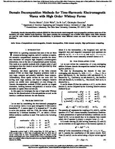
where λ is a parameter that defines the ’infectivity’ of the epidemics. Similar models are commonly used in epidemiology to assess the probability of infection as a function of the exposition time to a given pathogen [10]. B. K-Shell Decomposition The k-shell (or k-core) decomposition method has been introduced as a tool to analyse the structural properties of large graphs [3]. Definition 1: Given a graph G = {V, E}, the subgraph H = {C, E|C}, induced by C ⊆ V is a k–core of G if and only if it is the maximal subgraph of G such that the degree of every node in H is at least k. Definition 2: A node v ∈ V is said to belong to the ks shell (or to have k–shell index ks ) if and only if it belongs to the ks –core but not to the (ks + 1)–core. The k–shell decomposition of a graph can be performed iteratively. The degree of a node is defined as the number of arcs incident on a given vertex. Nodes of degree one have k–shell index equal to one. We prune all these nodes and the links incident on them from the graph. Nodes that have degree one on the reduced graph are assigned k–shell index of one and recursively pruned. The same is done for k = 2 and so on, until all nods are pruned from the graph. Remark 1: The k–shell decomposition of a graph G can be computed in O(N + E), where N is the number of nodes and E is the number of edges. [11] Remark 2: The k–shell decomposition can be computed in a decentralized fashion. To compute its own k–shell index, each node needs to know only the degree of its neighbours. In general, k–shell decomposition is useful for understanding both (i) the presence of hierarchical structures in a graph (ii) clusters of tightly connected nodes. The k–shell index is based only the degree of nodes in a graph. However, it provides more information on the role played by a node in the graph than the raw degree. As an example, consider a star–shaped topology. No matter what the degree of the central node, its k–shell index is equal to one. This reflects the fact that a star– shaped graph has a “flat” structure. Many structures found in the real-world present instead a very rich structure; k–shell decomposition provides a tool for studying and visualising it [4], [7]. An example of k–shell decomposition is reported in Fig. 1. Generalisations of the k–shell concept are presented in [12] based on a vertex property function. A number of possible options are discussed, with focus in particular on graphs with weighted links, where the vertex property function can be computed as a function of the weights associated to the links incident on that node. It is also proved that vertex property

500

Fig. 1: K–shell decomposition for a sample graph.

functions respecting a monotonicity property allow the corresponding generalised k–cores to be computed iteratively, as described above for the (standard) k–shell index. C. The “Flat” Model The first method we introduce for computing the k–core on a dynamic network is based on the use of a time windowing method to build, starting from a contact trace, a graph Gf lat (τ ). In such a graph, two nodes i and j are linked with an edge if and only if they meet within an interval of duration τ . (For the sake of simplicity we omit from the notation the starting point in time from which the interval of duration τ is computed.) We can then apply to the resulting Gf lat (τ ) graph the standard k–shell decomposition. We call this method the “flat” one, in that it does not account for the duration of single meetings among pairs of nodes. In other terms, all contacts are considered to have the same probability of leading to an infection, regardless of their respective duration. Such a model is expected to provide reasonably good results in situations in which the values of contact duration have a limited variance. Similarly, this method works well in situations in which the duration of contact is very long, such that the probability of infection is close to one, regardless of the actual value of the contact duration. On the contrary, in situations in which the contact duration follows an heavy-tail distribution or in general presents a large variance, such a method can overestimate the importance of short contacts. This technique can be applied using local information only. In a decentralized implementation, each node maintains a list of the nodes it has met within the previous τ seconds. Upon meeting with a node, the current values of the degree (nodes with which a meeting has taken place in the last τ seconds) are exchanged. The k–shell index is then re–computed according to the procedure outlined above. Clearly, the resulting k–shell index varies over time; in general the duration of the time interval τ should be taken large enough so as to capture the statistical properties of the contact pattern (assuming it is time–stationary and ergodic). D. The “Rich” Model The technique introduced in the previous section does not account for the duration of contacts. Yet, the duration of a

contact may have a relevant impact on the probability of an infection propagating from one node to another. In this section, we present a refined method, which accounts for the duration and defines a different metric to be considered. We first introduce a generalized k–shell index (applicable to nodes with weighted nodes and links), and then we discuss how to apply it to our framework. Definition 3 ((P, ϕ)–Generalized k–shell Decomposition): We assume a graph G where a real–valued number is assigned to each node. We term such a value the potential of the node and denote by P (i), i ∈ V. Further, we associate a real–valued number to each edge. We term such a value the capacity of the link and denote it by ϕ(e), e ∈ E. A node i is said to belong to the (P, ϕ)–generalized kc –core if and only if it has at least kc neighbours satisfying: P (j) · ϕ(i, j) ≥ kc ,

(3)

where j ∈ N (i) and ϕ(i, j) is the capacity of the link connecting nodes i and j. A node is said to belong to the (P, ϕ)–generalized ks –shell if it belongs to the (P, ϕ)– generalized ks –core but not to the (P, ϕ)–generalized (ks +1)– core. Remark 3: By taking P (i) = k(i) and ϕ(i, j) = 1 if (i, j) ∈ E we obtain the standard k–shell decomposition. Remark 4: The generalized k–shell index introduced in this paper does not fit the generalisation, based on vertex property function, presented in [12]. Remark 5: The (P, ϕ) generalized k–shell index can be computed in an iterative way, using the same process introduced in the previous section for the standard k–shell index. Remark 6: The (P, ϕ) generalized k–shell index can be computed in a decentralized fashion. Each node needs to be aware of the potential of its neighbours and of the capacity of the links incident on it. In the second model, that we term the “rich” one (in that it accounts also for the information on links duration) we take P (i) = k(i) and associate to each link a capacity ϕ(i, j) defined as the multiple (by a given factor Ψ) of the fraction of time nodes i and j are connected within a window of duration τ . In the remainder of the paper, we will refer to the resulting index simply as the ’generalized k–shell index’. The rationale behind such a choice is the following. By taking P (i) = k(i) we account for the importance of the number of nodes that can be potentially infected during a given time interval of duration τ . At the same time, by accounting for the average fraction of time two nodes are connected we weigh the importance of a contact by its duration. It is worth remarking the importance, in our framework, of the multiplicative coefficient Ψ. The (P, ϕ)–generalized k– shell decomposition method described above presents indeed a normalization issue. In fact, in (3) we are comparing a quantity (i.e., P (j) · ϕ(i, j)) to the number of neighbours. If such a quantity takes low values (e.g., below 1), all nodes will end up with a generalized k–shell index equal to one. At the same time, if the values taken by the product are too large, an

501

K−Shell Index Autocorrelation Function

unnecessary spread in the resulting generalized indexes may appear. As for the flat model, also in the rich one the resulting shell index varies over time, as only the events having taken place within the last τ s are considered in the computation. In the following section we will evaluate numerically the variability over time of the resulting generalized k–shell index. III. N UMERICAL R ESULTS Numerical emulations were carried out in order to assess:

1

0.8

0.6

0.4

0.2

0

1) The evolution over time of the resulting k–shell index, given that the two methods introduced are based on a time windowing operation; 2) The ability of the proposed models to characterise the ability of single nodes to spread an epidemic in the network, using synthetically generalised contact traces; 3) The applicability to real–world contact traces. We implemented the techniques presented in the previous section in Matlab and tested them against a number of contact traces. We used both synthetic and real–world traces. As far as synthetically generated traces are concerned, the settings used are reported in Tab. I, unless otherwise specified. The traces are generated as follows. A fixed number of contacts is considered. The time elapsed between two subsequent contacts (intrameeting time [9]) is generated according to an exponential distribution. For each contact, the IDs of the nodes and the duration of the contact are drawn according to a given distribution. Two parameters were varied in terms of mobility pattern features, resulting in four different cases. The first parameter we varied was the statistical distribution of the contact duration, where we considered two options: exponential and Pareto (with shape parameter α = 2). The first option corresponds to a situation where contacts have a “typical” duration, with rather limited variability. The second case corresponds to a situation where the contact duration may span a very wide range, presenting a large variability. The second parameter we varied was the distribution of the marks σn = (i, j), denoting the IDs of the nodes meeting at a contact opportunity. In the homogeneous case, all pairs of nodes have the same probability of getting in contact, P[σn = (i, j)] = N ·(N1 −1) ∀i, j, n. In the heterogeneous case, the probability associated to a given mark was drawn from a Pareto distribution (with mean 10 and shape parameter α = 2) and then normalized. The homogeneous case models situations where all nodes follow similar mobility patterns, so that the probability of any pair getting in touch is the same. The heterogeneous case reflects highly skewed situations, in which some pairs of nodes meet much more often than others. For a given trace, the k–shell index and the generalized k– shell index were computed. For the latter one, a multiplicative coefficient Ψ = 2000 was used. For both cases, a time window of duration τ = 120000 s was considered. The number of contacts of each node (degree) was also traced.

0

1

2

3

Time Lag (s)

4

5

6 6

x 10

Fig. 2: Autocorrelation function of the k–shell index as a function of time, τ = 200, 000s.

A. Temporal Evolution We first studied the temporal variation of the k–shell index, computed. Results are reported only for the flat model. Similar findings resulted also for the rich model. We considered a sliding window approach, according to which the k–shell index is re-computed every ∆ s, using the contacts having taken place within the last τ s. This gives rise, for a given trace, to a vector of sequences, where each sequence denotes the temporal evolution of the k–shell index of each node. We computed the autocorrelation function associated to each sequence, and averaged it over the set of nodes. Results are reported for exponentially distributed intrameeting times and exponentially distributed contact duration. Results are similar for the other three types of synthetic traces considered. We fixed ∆ = 30, 000 s and first set τ = 200, 000. The resulting autocorrelation function is reported, as a function of the time lag, in Fig: 2. As it can be seen, the correlation decays rather slowly over time, implying that the k–shell index evolution is rather slow. As the trace we are considering is time–stationary, this also reflects the fact that with the considered value of τ the time windowing method is able to capture well the statistical property of the dynamic network. We also analysed in depth the changes over subsequent time windows. Results showed that, for the given set of parameters, the variability is rather small, i.e., the k–shell index tends to present small variations over subsequent time windows. As an example, we depicted in Fig. 3 the probability of a given node to change from a shell of index x to a shell of index y in the successive time interval of duration τ . The dark areas represent probabilities close to one, whereas light gray areas represent little likely transitions. As it can be seen, dark areas are clustered around the main diagonal, which shows that small variations only take place with large probability. In order to assess the importance of choosing a long enough time window interval τ , we run the same experiments considering different values for such a parameter. In Fig. 4 and Fig. 5 we reported the results obtained using τ = 40, 000 s. We can notice that (i) the autocorrelation function decays faster

502

Parameter Number of nodes Number of contacts generated Distribution of IDs Intrameeting time distribution Mean intrameeting time Contact duration distribution Mean contact duration Generalized k–shell index multiplicative coefficient (Ψ) Infectivity coefficient (λ) Window size (τ ) Epidemic duration

Value 300 20000 uniform, normalized Pareto (α = 2) Exponential 90 s Exponential, Pareto (α = 2) 30 s 2000 0.07 120000 s 120000 s

TABLE I: Settings used for simulation purposes.

16

1

1

6

1E−1

1E−1

14

1E−2

K−Shell Index at Time t+∆

K−Shell Index at Time t+∆

5 12 1E−3 10 1E−4 8

1E−5

6

1E−6 1E−7

4

1E−3

4

1E−4 3

1E−5 1E−6

2 1E−7 1E−8

1

1E−8

2

1E−2

1E−9

1E−9 0

0

2

4

6

8

10

12

14

0

16

K−Shell Index at Time t

0

1

2

3

4

5

6

K−Shell Index at Time t

Fig. 5: Graphical representation of the probability of moving from a k–shell index x to a k–shell index y between subsequent time windows, τ = 40, 000s.

over time (ii) the dark areas in the colormap graph are less clustered along the main diagonal, implying a larger variability for the k–shell index between subsequent windows.

Initially, one single node was taken to be infected. Meetings involving infected nodes lead to an infection with probability that depends from the contact duration according to (2). The number of infected nodes after 120000 s from the starting time was traced. The procedure was repeated taking as initial spreader all nodes in the networks. For the four cases described above, the following figures were drawn: (i) Network structure according to the k–shell index. (Nodes with a higher k–shell represented with larger markers and placed in the higher part of the figure; edges connecting nodes represent a contact having taken place.) This is used to depict the resulting network structure. (ii) Network structure according to the generalized k–shell index. (Same procedure as for the case (i)). (iii) Fraction of nodes infected as a function of the k–shell index. A cross was drawn for the fraction of infected nodes starting from a given node i, plus the average fraction of nodes infected as a function of the k–shell index. The number of crosses in the graph equals the number of nodes in the network, i.e., 200. (iv) Fraction of nodes infected as a function of the generalized k–shell index. A cross was drawn for the fraction of infected nodes starting from a given node i, plus the

K−Shell Index Autocorrelation Function

Fig. 3: Graphical representation of the probability of moving from a k–shell index x to a k–shell index y between subsequent time windows, τ = 200, 000s.

1

0.8

0.6

0.4

0.2

0

0

1

2

3

4

5

Time Lag (s)

6 6

x 10

Fig. 4: Autocorrelation function of the k–shell index as a function of time, τ = 40, 000s. B. Network Structure and Spreading Efficiency We then emulated, for each trace, the spreading of an epidemic as follows. First, a random starting point was chosen in the trace according to a uniform distribution in [0, 50000] s.

503

average fraction of nodes infected as a function of the generalized k–shell index. (v) Fraction of nodes infected as a function of the node degree. A cross was drawn for the fraction of infected nodes starting from a given node i, plus the average fraction of nodes infected as a function of the node degree. The resulting outcomes are reported in Fig. 6–9 for a given trace. While the results reported refer to the outcomes of a single run, their behaviour was consistent across multiple runs. Some observations can be drawn: 1) The rich model leads to network structures whereby nodes of high index are less than in the corresponding flat model. In the flat model, a large fraction of nodes achieves large k–shell index (close to the maximal one). 2) The node degree is not a good indicator of the ability of the node to effectively spread an epidemic in the network, as represented by its unstable and non–monotonic behaviour in all the four cases considered. 3) For exponentially distributed contact durations, both the k–shell and the generalized k–shell indexes represent a good metric for understanding the “spreading power” of a given node, as nodes with higher index tend to lead to a larger fraction of nodes getting infected within a given deadline. 4) When the contact duration follows an heavy–tail distribution (in our case: Pareto with shape parameter α = 2), the generalized k–shell index represents a more robust metric of the ability of a node to effectively spread an epidemic in the network. In this case indeed the fraction of infected nodes turns out to be a non–monotonic function of the k–shell index. C. Real–World Traces In order to assess the ability of our models to identify the most influential spreaders in dynamic complex networks, we also performed some simulation tests using real–world traces. Such traces usually come from experiments where a number of users, equipped with mobile phones supporting some form of short–range wireless communication, are traced for a given period of time. This is done by having nodes periodically sending out beacon messages, which contain their ID. Received beacons are stored at the receiving node. In this way it is possible to reconstruct the overall sequence of meetings among nodes. Log files, once filtered and properly anonymized, are usually released to the scientific community2. Among the various traces we experimented with, we report here result obtained using the trace coming from the Reality Mining initiative at MIT [13]. The data was gathered as follows. One hundred smartphones were distributed among students at MIT. Each phone was Bluetooth-enabled and contained software for tracing contacts with other Bluetooth devices. The experiment lasted nine months. 2 A variety of traces of this type can be found in the CRAWDAD repository, http://crawdad.cs.dartmouth.edu/.

We processed such a trace by removing spurious encounters, and limited our analysis to the first 200, 000 contacts. The resulting network consisted of 94 nodes, with an average intrameeting time of 83 s and an average contact duration of 35 minutes. Statistical analysis of the data features showed a large variability in intrameeting time, which followed an approximate power–law distribution with an exponential tail. It is worth remarking that the average duration of contacts is in this case much larger than the values we used for synthetically generated traces. This comes from the fact that the users in the experiments were all students, who turned out to spend a lot of time in contact (either because they were following the same class, studying in the same library etc.). We repeated for the MIT trace the same procedure carried out in the previous subsection for synthetically generated traces. We used λ = 0.0001 as infectivity rate, τ = 10, 000 s as window size and considered an epidemic of duration 30, 000 s. The results are reported in Fig. 10. The first thing that clearly emerges is that the flat and rich model provides very different results in terms of the structure. This is due to the fact that in the MIT dynamic network there is a node which acts as a central ’hub’, meeting often many of the other nodes. This implies that the network has a star–like structure. The k–shell decomposition in this case treats the hub as its leaves, resulting in a low variability in the k–shell index (which spans the interval [0, 6]. The generalised k–shell instead, by accounting for the duration of meetings each node got involved in, tends to highly estimate the relevance of the hub in the system, which turns out to have a generalised k–shell index of 47. (Remark: this effect can be partially alleviated by using a different value for the Ψ parameter in the computation of the generalised k– shell index.) As far as the ability of the indexes to identify most influential spreaders, results in 10.c–e show that there is not much difference, in this case, among the various metrics. IV. C ONCLUSION

AND

F UTURE W ORK

Recent works have highlighted the ability of the k–shell index to describe the ability of a node to effectively spread an epidemic in a complex network [1]. This work represents an attempt to extend such an approach to dynamic networks, where the spreading dynamics is driven by a contact process describing potential interactions among nodes. In particular, we introduced two methods, both based on a time windowing approach, for associating a shell index to nodes. The evolution over time of the proposed methods, as well as their ability to effectively identify good spreaders have been assessed through a simulation campaign involving both synthetic as well as real– world traces. Two directions appear of interest. The first one relates to the use of other generalised k–shell concepts [12] to better deal with the properties of real–world contact traces. The second one relates to the application of the proposed techniques to the design of effective protocols for epidemically disseminating data in intermittently connected wireless networks. Schemes proposed in the literature make use of betweenness centrality [14], [15] or of nodes degree [16] for understanding the

504

1 0.9

1

0.8 0.7

0.8

0.6 0.6

0.5 0.4

0.4

0.3 0.2

0.2

0.1 0

0

0.1

0.2

0.3

0.4

0.5

0.6

0.7

0.8

0.9

0

1

0

0.2

0.3

0.4

0.5

0.6

0.7

0.9

0.8

0.8

0.6 0.5 0.4 0.3 0.2 0.1 0

Fraction of Infected Nodes

0.9

0.8 0.7

0.7 0.6 0.5 0.4 0.3 0.2 0.1

1

2

3

4

5

6

7

8

9

10

0

11

0.8

0.9

1

(b) Network structure, rich model

0.9

Fraction of Infected Nodes

Fraction of Infected Nodes

(a) Network structure, flat model

0.1

0.7 0.6 0.5 0.4 0.3 0.2 0.1

0

1

2

K−Shell Index

3

4

5

6

7

0

8

0

2

4

6

8

Generalized K−Shell Index

(c) Fraction of infected nodes vs. k–shell index

10

12

14

16

18

Node degree

(d) Fraction of infected nodes vs. generalized k–shell index

(e) Fraction of infected nodes vs. node degree

Fig. 6: Exponentially distributed contact duration, homogeneous marks distribution. 1

1

0.9

0.9

0.8

0.8

0.7

0.7

0.6

0.6

0.5

0.5

0.4

0.4

0.3

0.3

0.2

0.2

0.1 0

0.1

0

0.1

0.2

0.3

0.4

0.5

0.6

0.7

0.8

0.9

0

1

0

(a) Network structure, flat model

0.2

0.3

0.4

0.5

0.6

0.5

0.4

0.3

0.2

0.6

0.5

0.4

0.3

0.2

0.1

0.1

0

0

1

2

3

4

5

6

7

8

9

10

11

K−Shell Index

(c) Fraction of infected nodes vs. k–shell index

0.8

0.9

1

0.7

Fraction of Infected Nodes

0.6

0.7

(b) Network structure, rich model

0.7

Fraction of Infected Nodes

Fraction of Infected Nodes

0.7

0.1

0.6

0.5

0.4

0.3

0.2

0.1

0

1

2

3

4

5

6

7

Generalized K−Shell Index

(d) Fraction of infected nodes vs. generalized k–shell index

0

0

2

4

6

8

10

12

14

16

18

20

Node degree

(e) Fraction of infected nodes vs. node degree

Fig. 7: Pareto distributed contact duration, homogeneous marks distribution.

goodness of a node as a potential relay of information. We believe that using k–shell index (either standard or generalized) can help in devising better routing schemes. In this respect,

it is important to remark that both metrics can be computed in a decentralized way, requiring no global knowledge on the overall network structure.

505

1

1

0.9

0.9

0.8

0.8

0.7

0.7

0.6

0.6

0.5

0.5

0.4

0.4

0.3

0.3

0.2

0.2

0.1 0

0.1

0

0.1

0.2

0.3

0.4

0.5

0.6

0.7

0.8

0.9

0

1

0

0.2

0.3

0.4

0.5

0.6

0.7

1

1

0.9

0.9

0.7 0.6 0.5 0.4 0.3 0.2

0.8 0.7 0.6 0.5 0.4 0.3 0.2

0.1

0.1

0

0

0

1

2

3

4

5

6

7

8

9

10

Fraction of Infected Nodes

1

0.8

0.8

0.9

1

(b) Network structure, rich model

0.9

Fraction of Infected Nodes

Fraction of Infected Nodes

(a) Network structure, flat model

0.1

0.8 0.7 0.6 0.5 0.4 0.3 0.2 0.1

0

1

2

K−Shell Index

3

4

5

6

7

0

8

0

2

4

6

Generalized K−Shell Index

(c) Fraction of infected nodes vs. k–shell index

8

10

12

14

16

Node degree

(d) Fraction of infected nodes vs. generalized k–shell index

(e) Fraction of infected nodes vs. node degree

Fig. 8: Exponentially distributed contact duration, heterogeneous marks distribution. 1

1

0.9

0.9

0.8

0.8

0.7

0.7

0.6

0.6

0.5

0.5

0.4

0.4

0.3

0.3

0.2

0.2

0.1 0

0.1

0

0.1

0.2

0.3

0.4

0.5

0.6

0.7

0.8

0.9

0

1

0

0.2

0.3

0.4

0.5

0.6

0.7

0.8

0.7

0.7

0.5 0.4 0.3 0.2

0.6 0.5 0.4 0.3 0.2

0.1

0.1

0

0

0

1

2

3

4

5

6

7

8

9

10

K−Shell Index

(c) Fraction of infected nodes vs. k–shell index

Fraction of Infected Nodes

0.8

0.7 0.6

0.8

0.9

1

(b) Network structure, rich model

0.8

Fraction of Infected Nodes

Fraction of Infected Nodes

(a) Network structure, flat model

0.1

0.6 0.5 0.4 0.3 0.2 0.1

0

1

2

3

4

5

6

7

Generalized K−Shell Index

(d) Fraction of infected nodes vs. generalized k–shell index

0

0

2

4

6

8

10

12

14

16

18

Node degree

(e) Fraction of infected nodes vs. node degree

Fig. 9: Pareto distributed contact duration, heterogeneous marks distribution.

ACKNOWLEDGMENT

R EFERENCES

This work has been supported by the EC within the framework of the EPIWORK project ICT-FET-COSI-ICT-FP7231807, www.epiwork.eu.

[1] M. Kitsak, L. K. Gallos, S. Havlin, F. Liljeros, L. Muchnik, H. E. Stanley, and H. A. Makse, “Identifying influential spreaders in complex networks,” 01 2010, http://arxiv.org/abs/1001.5285.

506

1

1

0.9

0.9

0.8

0.8

0.7

0.7

0.6

0.6

0.5

0.5

0.4

0.4

0.3

0.3

0.2

0.2

0.1 0

0.1

0

0.1

0.2

0.3

0.4

0.5

0.6

0.7

0.8

0.9

0

1

0

0.2

0.3

0.4

0.5

0.6

0.7

0.8

0.7

0.7

0.5 0.4 0.3 0.2

0.6 0.5 0.4 0.3 0.2

0.1

0.1

0

0

0

1

2

3

4

5

6

7

K−Shell Index

Fraction of Infected Nodes

0.8

0.7 0.6

0.9

1

0.6 0.5 0.4 0.3 0.2 0.1

0

5

10

15

20

25

30

35

40

45

0

Generalized K−Shell Index

(c) Fraction of infected nodes vs. k–shell index

0.8

(b) Network structure, rich model

0.8

Fraction of Infected Nodes

Fraction of Infected Nodes

(a) Network structure, flat model

0.1

(d) Fraction of infected nodes vs. generalized k–shell index

0

5

10

15

20

25

30

35

40

Node degree

(e) Fraction of infected nodes vs. node degree

Fig. 10: MIT Reality Mining contact trace.

[2] G. Canright and K. Engø-Monsen, “Spreading on networks: a topographic view,” in Proc. of ECCS, Paris, 2005. [3] S. B. Seidman, “Network structure and minimum degree,” Social Networks, vol. 5, pp. 269–287, 1983. [4] S. Carmi, S. Havlin, S. Kirkpatrick, Y. Shavitt, and E. Shir, “New model of internet topology using k-shell decomposition,” CoRR, vol. abs/cs/0607080, 2006. [5] V. Colizza, M. Barthelemy, A. Barrat, and A. Vespignani, “Epidemic modeling in complex realities,” CR Biologies, vol. 330, pp. 364–374, 2007. [6] E. Yoneki, P. Hui, and J. Crowcroft, “Wireless epidemic spread in dynamic human networks,” in Bio-Inspired Computing and Communication. Springer, 2008, pp. 116–132, lNCS 5151. [7] J. I. Alvarez-Hamelin, L. Dall’Asta, A. Barrat, and A. Vespignani, “Kcore decomposition of Internet graphs: hierarchies, self-similarity and measurement biases,” Networks and Heterogeneous Media, vol. 3, pp. 271–293, 2008. [8] F. Baccelli and P. Bremaud, Elements of Queueing Theory. Berlin: Springer–Verlag, 1994. [9] I. Carreras, D. Miorandi, and I. Chlamtac, “A simple model of contact patterns in delay-tolerant networks,” Springer/ACM Wireless Networks, vol. 16, pp. 851–862, Mar. 2010. [10] T. Smieszek, “A mechanistic model of infection: why duration and intensity of contacts should be included in models of disease spread,” Theoretical Biology and Medical Modelling, vol. 6, Nov. 2009. [11] V. Batagelj and M. Zaversnik, “An O(m) algorithm for cores decomposition of networks,” CoRR, vol. cs.DS/0310049, 2003. [Online]. Available: http://arxiv.org/abs/cs.DS/0310049 [12] ——, “Generalized cores,” CoRR, vol. cs.DS/0202039, 2002. [Online]. Available: http://arxiv.org/abs/cs.DS/0202039 [13] N. Eagle and A. Pentland, “Reality Mining: sensing complex social systems,” Personal and Ubiquitous Computing, vol. 10, pp. 255–268, May 2006. [14] E. M. Daly and M. Haahr, “Social network analysis for routing in disconnected delay-tolerant MANETs,” in Proc. of ACM MobiHoc, 2007. [15] P. Hui, J. Crowcroft, and E. Yoneki, “Bubble rap: Social-based forwarding in delay tolerant networks,” in Proc. of ACM MobiHoc, 2008. [16] A. Picu and T. Spyropoulos, “Minimum expected *-cast time in dtns,”

507

in Proc. of BIONETICS. pp. 103–116.

Avignon, France: LNICST, Springer, 2009,