Deconvolution with correct sampling P. Magain1
arXiv:astro-ph/9704059v2 14 Oct 1997
Institut d’Astrophysique, Universit´e de Li`ege, 5, avenue de Cointe, B–4000 Li`ege Belgium email:
[email protected]
F. Courbin Institut d’Astrophysique, Universit´e de Li`ege, 5, avenue de Cointe, B–4000 Li`ege Belgium email:
[email protected] URA 173 CNRS-DAEC, Observatoire de Paris, F-92195 Meudon Principal CEDEX, France
S. Sohy Institut d’Astrophysique, Universit´e de Li`ege, 5, avenue de Cointe, B–4000 Li`ege Belgium email:
[email protected]
ABSTRACT A new method for improving the resolution of astronomical images is presented. It is based on the principle that sampled data cannot be fully deconvolved without violating the sampling theorem. Thus, the sampled image should not be deconvolved by the total Point Spread Function, but by a narrower function chosen so that the resolution of the deconvolved image is compatible with the adopted sampling. Our deconvolution method gives results which are, in at least some cases, superior to those of other commonly used techniques : in particular, it does not produce ringing around point sources superimposed on a smooth background. Moreover, it allows to perform accurate astrometry and photometry of crowded fields. These improvements are a consequence of both the correct treatment of sampling and the recognition that the most probable astronomical image is not a flat one. The method is also well adapted to the optimal combination of different images of the same object, as can be obtained, e.g., from infrared observations or via adaptive optics techniques.
Subject headings: Methods: Numerical - Observational - Data analysis
1
Maˆıtre de Recherches au Fonds National de la Recherche Scientifique (Belgium)
–2– 1.
Deconvolution
Any recorded image is blurred whenever the instrument used to obtain it has a finite resolving power : for example, the image of a point source seen through a telescope has an angular size which is inversely proportional to the diameter of the primary mirror. If the instrument is ground-based, the image is additionally degraded by the turbulent motions in the earth’s atmosphere. Much effort is presently devoted to the improvement of the spatial resolution of astronomical images, either via the introduction of new observing techniques (e.g. interferometry or adaptive optics, see L´ena 1996, Enard et al. 1996) or via a subsequent numerical processing of the image (deconvolution). It is, in fact, of major interest to combine both methods to reach an even better resolution. An observed image may usually be mathematically expressed as a convolution of the original light distribution with the “total instrumental profile” — the latter being the image of a point source obtained with the instrument considered, including the atmospheric perturbation (seeing) if relevant. The total blurring function is called the Point Spread Function (PSF) of the image. Thus, the imaging equation may be written : d(~x) = t(~x) ∗ f (~x) + n(~x)
(1)
where f (~x) and d(~x) are the original and observed light distributions, t(~x) is the total PSF and n(~x) the measurement errors (noise) affecting the data. In addition, on all modern light detectors (e.g. CCDs whose pixels have finite dimensions), the observed light distribution is sampled, i.e. known only at regularly spaced sampling points. The imaging equation for a sampled light distribution then becomes : di =
N X
tij fj + ni
(2)
j=1
where N is the number of sampling points, dj , fj , nj are vector components giving the sampled values of d(~x), f (~x), n(~x) and tij is the value at point j of the PSF centered on point i. The aim of deconvolution may be stated in the following way : given the observed image d(~x) and the PSF t(~x), recover the original light distribution f (~x). Being an inverse problem, deconvolution is also an ill-posed problem, and no unique solution can be found, especially in the presence of noise. This is due to the fact that many light distributions are, after convolution with the PSF, compatible within the error bars with the observed image. Therefore, regularization techniques have to be used in order to select a plausible solution amongst the family of possible ones and a large variety of deconvolution methods have been proposed, depending on the way this particular solution is chosen. A typical method is to minimize the χ2 of the differences between the data and the convolved model, with an additional constraint imposing smoothness of the solution. fj is then the light distribution which minimizes the function : S1 =
N X 1 i=1
σi2
N X
j=1
2
tij fj − di + λ H(f1 , · · · , fN )
(3)
–3– where the first term in the sum is the χ2 with σi the standard deviation of the image intensity measured at the ith sampling point, H is a smoothing function and λ a Lagrange parameter which is determined so that the reconstructed model is statistically compatible with the data (χ2 ≃ N ). PN P If H(f1 , · · · , fN ) = N j=1 fj , one i=1 pi ln pi , with pi the normalized flux at point i, pi = fi / obtains the so-called maximum entropy method for image deconvolution (Narayan and Nityananda 1986, Skilling and Bryan 1984). In order to choose the correct answer in the family of possible solutions to this inverse problem, it is also very useful to consider any available prior knowledge. One such prior knowledge is the positivity of the light distribution : no negative light flux can be recorded, so that all solutions with negative values may be rejected. The maximum entropy method automatically ensures positivity of the solution. This is also the case, under certain conditions, for other popular methods, such as the Richardson-Lucy iterative algorithm (Richardson 1972, Lucy 1974). Most of the known deconvolution algorithms suffer from a number of weak points which strongly limit their usefulness. The two most important problems in this respect are the following : (1) traditional deconvolution methods tend to produce artefacts in some instances (e.g. oscillations in the vicinity of image discontinuities, or around point sources superimposed on a smooth background) ; (2) the relative intensities of different parts of the image (e.g. different stars) are not conserved, thus precluding any photometric measurements. In the next sections, we identify a plausible cause of these problems and show how to circumvent it.
2.
Sampling
The sampling theorem (Shannon 1949, Press et al. 1989) determines the maximal sampling interval allowed so that an entire function can be reconstructed from sampled data. It states that a function whose Fourier transform is zero at frequencies larger than a cutoff frequency ν0 is fully specified by values spaced at equal intervals not exceeding (2 ν0 )−1 . In practice, for functions whose Fourier transform does not present such a cutoff frequency, ν0 may be taken as the highest frequency at which the Fourier transform emerges from the noise. The imaging instruments are generally designed so that the sampling theorem is approximately fulfilled in average observing conditions. A typical sampling encountered is ∼ 2 sampling intervals per Full Width at Half Maximum (FWHM) of the PSF (this does certainly not ensure good sampling for high signal-to-noise (S/N) images, but is roughly sufficient at low S/N). The main problem with classical deconvolution algorithms is the following : if the observed data are sampled so that they just obey the sampling theorem, the deconvolved data will generally violate that same theorem. Indeed, increasing the resolution means recovering highest Fourier frequencies, thus increasing the cutoff frequency, so that the correct sampling becomes denser. One might object that some deconvolution algorithms, which allow a different sampling in the deconvolved image, could overcome this problem : it would be possible to keep a correct sampling by shortening the sampling interval. This is however an illusory solution, since the only limit on the frequency components present in an arbitrary image comes from the PSF of the instrument
–4– used to record it. Removing the effect of the PSF would allow the presence of arbitrary high frequency components, and thus an infinitely small sampling interval would have to be used. This is particularly true if the image contains point sources, which is generally the case for astronomical images. Indeed, the angular diameters of most stars (≪ 0.001 arcsec) are so small compared to the sampling interval (∼ 0.1 arcsec) that they may be considered as point sources (“δ-functions”). In such an instance, it would be hopeless to reduce the sampling interval in an attempt to obtain a good sampling of such “δ-functions”. This is one of the sources of some of the artefacts present in the deconvolved images and, in particular, of the “ringing” around point sources superimposed on a diffuse background. The origin of this “ringing” may be understood in the following way. Let us assume that we have a continuous (i.e. not sampled) noise-free image of a field containing point sources, and observed with an instrument having a known PSF. For simplicity, we restrict our considerations to one-dimensional images. If we can perfectly deconvolve this image, we shall obtain a solution f (x) in which each point source is represented by a Dirac δ-function. Now, let us assume that we have the same image, but sampled on N points, with a sampling step ∆x. The Fourier transform of its deconvolution may be obtained from the Fourier transform F (ν) of the continuous deconvolution in the following way : repeat periodically F (ν) with the Nyquist frequency νN y = (2∆x)−1 , take the sum of all these periodical replicas at each frequency point, isolate one period and sample it on N equally spaced frequency points. Isolating one period means multiplying the Fourier transform by a rectangular (“box”) function which equals 1 in an interval of length νN y and 0 outside. Now, a convolution in the image domain translates into a simple product in the Fourier domain, and vice-versa. This multiplication by a box function in the Fourier domain is thus equivalent, in the image domain, to a convolution by the Fourier transform of the box function, which is a function of the form sin x/x. The solution of the deconvolution problem for a sampled image with point sources is thus the (sampled) convolution of the exact solution f (x) with a function of the form sin x/x. Each δ-function is thus replaced by an oscillatory sin x/x function, which explains the ringing. Another, more intuitive, explanation of the same effect is the following. If a point source is located between two sampling points (as will generally be the case), in order to correctly reproduce its position, the deconvolution algorithm will have to distribute its intensity over several sampling points. But, then, the width of the source will be too large and ringing will appear as the algorithm attempts to decrease the intensity on the edges of the reconstructed source, in order to keep the convolved model as close as possible to the observed data. In fact, it is not possible to correctly reproduce both the position and the width of a sampled point source. To reproduce the zero width, the full signal must be concentrated on a single sampling point. On the other hand, to reproduce the position with a precision which is better than the sampling interval, the signal has to be distributed over several points.
–5– 3.
Solution
The correct approach to this sampling problem is thus not to deconvolve with the total PSF t(~x), but rather with a narrower function s(~x) chosen so that the deconvolved image has its own PSF r(~x) compatible with the adopted sampling. These three functions are simply related by : t(~x) = r(~x) ∗ s(~x)
(4)
Note that a similar decomposition was proposed, in a completely different context (reduction of artefacts in maximum-likelihood reconstructions for emission tomography), by Snyder et al. (1987). The shape and width of r(~x) can be chosen by the user. The only constraint is that Eq. (4) admits a solution s(~x). The function s(~x) by which the observed image has to be deconvolved is thus obtained as the deconvolution of the total PSF t(~x) by the final PSF r(~x). Of course, the sampling interval of the deconvolved image does not need to be equal to the sampling interval of the original image, so that r(~x) may be much narrower than t(~x), even if the original sampling would not allow it. Choosing a sufficiently narrow r(~x) effectively insures that Eq. (4) will admit a solution s(~x). Note also that, contrary to other traditional methods (the success of which depends crucially on the effectiveness of the positivity constraint), we have no positivity constraint on the PSFs r(~x) and s(~x). Thus, the deconvolution algorithm should not attempt to determine the light distribution as if it were obtained with an ideal instrument (e.g. a space telescope with a primary mirror of infinite size). This is forbidden as long as the data are sampled. Rather, the aim of deconvolution should be to determine the light distribution as if it were observed with a better instrument (e.g. a 10 m space telescope). Deconvolution by s(~x) ensures that the solution will not violate the sampling theorem. It also has a very important additional advantage : if the image contains point sources, their shape in the deconvolved image is now precisely known : it is simply r(~x). This is a very strong prior knowledge, and it may be used to constrain the solution f (~x), which can now be written : f (~x) = h(~x) +
M X
ak r(~x − ~ck )
(5)
k=1
where M is the number of point sources, for which ak and ~ck are free parameters corresponding to their intensities and positions, and h(~x) is the extended component of the solution, i.e. generally a rather smooth background. We can use another prior knowledge to constrain the solution : we know that the background h(~x) can also be written as the convolution of some function h′ (~x) with the PSF of the solution r(~x) : h(~x) = r(~x) ∗ h′ (~x)
(6)
However, we cannot use that decomposition directly and determine h′ (~x) instead of h(~x) because h′ (~x) might violate the sampling theorem, even if it does not contain point sources. Rather, we may use this knowledge to impose smoothness of h(~x) on the scale length of r(~x).
–6– So, instead of regularizing the solution by a global function such as the entropy, we use a function imposing local smoothness of h(~x) on the known scale length. We thus choose the solution which minimizes the function : S2 =
N X 1 i=1
σi2
N X
j=1
sij hj +
M X
k=1
!
2
ak r(~xj −~ck ) − di + λ
N X i=1
hi −
with respect to the unknowns hi (i = 1, . . . , N ), ak and ~ck (k = 1, . . . , M ).
N X
j=1
2
rij hj
(7)
Although the smoothing term in the right-hand side of Eq. (7) will not force h(~x) to exactly obey Eq. (6), it essentially contains the Fourier components with frequencies higher than those of the deconvolved PSF r(~x). Minimizing this term will force the background component to contain only the frequencies compatible with r(~x) and, thus, with the adopted sampling. One additional improvement may be introduced. In general, the Lagrange multiplier λ is chosen so that χ2 ≃ N . This ensures that the fit is statistically correct globally. However, some regions of the image may be overfitted, and others may be underfitted. In practice, this will generally be the case : although the residuals will be correct on the average, they will systematically be too small in some parts of the image and too large in other parts. To avoid this problem, one may replace the smoothing function by : H(f1 , · · · , fN ) =
N X i=1
λi hi −
N X
j=1
2
rij hj
(8)
where λi is the value at the ith sampling point of a function λ(~x) which is chosen so that the residuals of the fit are correct locally, i.e. that they are statistically distributed with the correct standard deviation in any sub-part of the image. In practice, an image of the square of the normalized residuals (observed data minus convolved model, divided by sigma) is computed and then smoothed with an appropriate function, so that any value is replaced by a weighted mean on a neighborhood containing a few dozens of pixels. The parameter λ is then adjusted until this image is close to one everywhere.
4.
Examples
Our deconvolution program implements the ideas exposed in the preceding section. The light distribution aimed at is written as the sum of a smooth background plus a number of point sources. The sampling step of the deconvolved image is chosen, as well as the final PSF r(~x), compatible with this sampling (in general, we adopt a gaussian function, with a few pixels FWHM). Approximate values of the unknowns are chosen and the function S2 is computed, together with its derivatives with respect to all variables. The minimum of S2 is then searched for, using an algorithm derived from the classical conjugate gradient method (Press et al. 1989). The fit’s residuals are then computed and a check of their statistical correctness is performed. If this test is not satisfied, the Lagrange multiplier λ is replaced by a variable λ(~x) which is varied until the residuals conform to the statistical expectations.
–7– The present version of the program runs on PCs and workstations and can handle images of reasonable size (e.g., 256 × 256 pixels) containing up to several hundreds of stars. The main weakness of the present implementation is related to the conjugate gradient algorithm, which is not always able to find the global minimum of the function, especially when the number of point sources is large. We are presently working on a new optimization technique which would allow our method to be applied to the photometry of crowded fields with thousands of stars. It may not seem obvious at first sight to select the correct number of point sources to be included in the solution. However, the algorithm allows to constrain this number in a very efficient way : if too few point sources are entered, it will generally be impossible to obtain statistically correct residuals locally, in all sub-parts of the image. On the other hand, if too many point sources are considered, the algorithm will either attribute essentially the same position or negligible intensities to several of them. Our methodology is thus to model the data with the minimum number of point sources necessary to yield statistically correct residuals locally in all sub-parts of the image, in the sense described at the end of the preceding section. Figure 1 compares the results of our new deconvolution algorithm to those of three classical methods in the case of a simulated star cluster partly superimposed on a smooth background (e.g. a distant elliptical galaxy). The input point sources were selected from the observed image alone, without any prior knowledge of the exact solution. It is clear that our result is free from the artefacts present in the other methods and that it allows an accurate reconstruction of the original light distribution. Another important property of our technique is that it allows, contrary to the other ones, an accurate measurement of the positions and intensities of the point sources. This point will be discussed more extensively in the next section. An application to real astronomical data is shown on Fig. 2, which displays a mediocre resolution image of the “Cloverleaf”, a gravitationally lensed quasar (Magain et al. 1988), together with the deconvolved version, using a sampling interval twice as short. The four lensed images, which were unresolved in the original data, are completely separated after deconvolution. The deduced fluxes are fully compatible with those measured on higher resolution images and, although the original resolution is 1.3 arcsec only and the pixel size is 0.35 arcsec, the deduced image positions are accurate to 0.01 arcsec. Figure 3 illustrates the deconvolution of an image of the compact star cluster Sk 157 in the Small Magellanic Cloud (Heydari-Malayeri et al. 1989). The original image was obtained with the ESO/MPI 2.2m telescope at La Silla, in average seeing conditions (1.1 arcsec FWHM). While the original maximum entropy deconvolution (Heydari-Malayeri et al. 1989) allowed to resolve the cluster into 12 components, our new algorithm detects, from the same input data, more than 40 stars in the corresponding area. Another important application of our algorithm is the simultaneous deconvolution of different images of the same field. These images may be obtained with the same instrument or with different ones. The solution is then a light distribution which is compatible with all the images considered. Our technique even allows to let, e.g., the intensities of the point sources converge to different values in the different images, so that variable objects may be considered. This technique should be very useful for the photometric monitoring of variable objects in crowded fields or overimposed
–8– on a diffuse background (e.g. Cepheids in distant galaxies, gravitationally lensed QSOs,...). Figure 4 illustrates this simultaneous deconvolution on simulated images, the first of which has a good resolution but a poor S/N (as might be obtained with a space telescope) and the second one a low resolution and a high S/N (a typical image from a large ground-based telescope). Contrary to Lucy’s method (Hook and Lucy 1992) which is very sensitive to the noise present in one of the images, our technique allows to reliably recover both the high resolution of the space image and the hidden information content of the ground-based one. In the same spirit, our algorithm is well adapted to the processing of images obtained with infrared or adaptive optics techniques. In the latter, numerous short exposures of the same field are usually obtained, the shape of the mirror being continuously adapted to correct for atmospheric distortions. So, the observations consist in a number of images of the same field, each of them having its own PSF. Performing a simple sum results in an image whose spatial resolution is typical of the average observing conditions, while a simultaneous deconvolution not only allows to take count of the best conditions, but even results in an improved resolution by optimally combining the information content of the different images. A simple illustration of these considerations is provided by Fig. 5, which shows the simultaneous deconvolution of four adaptive-optics-like images of the same field, where the PSF as well as the image centering vary from one observation to the other. Of course, the PSF needs to be known for each individual observation, but only with an accuracy comparable to that of the observation itself.
5.
Astrometric and photometric accuracy
Traditional deconvolution methods are notoriously unable to give photometrically accurate results. Two main reasons for that are readily identified. First, as we have already mentioned, these methods generally produce rings when point sources are overimposed on a diffuse background. In fact, these rings tend to appear as soon as the positivity constraint is inefficient to inhibit them, that is, as soon as some flux is distributed around the point sources. This is most clearly seen when this flux is in the form of a smooth background, but the effect is also present if the flux is distributed among, e.g., a number of fainter stars. In this case, the rings around the star considered will interfere with the intensity in the neighbouring sources, and the photometry of the latter ones will be affected. A second photometric bias comes from the fact that, among the family of possible solutions to the inverse problem, most classical algorithms select, in one way or another, the smoothest one according to some criterion. These algorithms thus produce images where the peaks corresponding to point sources deviate as little as possible with respect to the background — provided, of course, that the model fits the data. This implies a systematic underestimate of the intensity peaks, and thus, a photometric bias. An example of these effects is illustrated by the deconvolution of an image of two point sources with varying separation. A simple image was constructed, with two point sources having an intensity ratio of 0.1, and convolved with a Gaussian PSF of 7 pixels FWHM, plus some gaussian
–9– noise so that the peak S/N ratio reaches 100. Figure 6 shows the deduced intensity ratio as a function of the source separation, as derived after deconvolution with the maximum entropy method. It clearly shows that the photometry is not preserved, even when the two stars are separated by nearly two FWHMs. For more details on the photometric accuracy of deconvolution algorithms (in the special case of HST images), see Busko (1994). Our algorithm naturally avoids these two biases. Indeed, the fact that the sampling theorem is obeyed in the deconvolved image, combined with the fact that no smoothing of the point sources is attempted, naturally ensure that no ringing is present around the star peaks, and that no bias will appear as a consequence of smoothing. This is illustrated in Fig. 7, which shows the results of a photometric test applied to a synthetic field containing 200 stars in a 128× 128 pixels image. The positions and central intensities were selected at random, and nearly all the stars are blended to varying degrees (197 stars out of 200 have the nearest neighbour within 2 FWHMs). Moreover, these stars are superimposed on a variable background. Figure 7 clearly shows that no systematic error is present, and that the intensities of all but the most severely blended objects are reproduced with errors compatible with the photon noise. Figure 8 illustrates the astrometric accuracy of our algorithm. For the brightest stars, the positional accuracy is generally better than 0.1 pixel, even in very severe blends. The positions of stars with a blend between 1 and 2 FWHM is generally accurate within 0.02 pixel at high S/N, and within 0.1 pixel otherwise. There exits another deconvolution algorithm which claims to achieve a high photometric quality, namely the so-called two-channel Lucy method (Lucy 1994, Hook and Lucy 1994). As our algorithm, the two-channel Lucy method is based on a decomposition of the deconvolved model into point sources and background. The main problem with that method is that, contrary to ours, the total PSF is used in the deconvolution, so that the sampling problem is avoided only if each point source is exactly centered on a pixel. To increase the accuracy, the model can use a finer pixel grid than the data. However, in high S/N cases, the model pixels will generally need to be very small if high accuracy is aimed at (which is normally the case in high S/N observations...). As an example, let us recall that the positions derived from our new algorithm for the different images of the Cloverleaf gravitational lens (Fig. 2) are accurate to 0.01 arcsec, which is 1/35 of a data pixel. To achieve the same accuracy with the two channel Lucy algorithm would require each original pixel to be devided in ∼ 35 × 35 ∼ 1000 finer pixels. This would rapidly result in huge data frames and computationally intractable problems. Another weakness of the two-channel Lucy method is that the point source positions have to be supplied by the user, and cannot be adjusted by the algorithm. So, no astrometry can be performed and, moreover, in the case of high S/N data with many point sources, it might require an unreasonably large number of trials for the user to find a fairly good estimate of the source positions. Finally, let us note that the user has to choose arbitrarily not only the number of iterations of the algorithm, but also a scale length for the smoothing of the background component. These choices are generally made by looking at the results. This approach can obviously give nice-looking
– 10 – results, but their scientific soundness may be questioned. On the contrary, the scale length for the smoothing of the background in our method is unambiguously fixed by the PSF r(~x) of the deconvolved image. A comparison of the two-channel Lucy method with our algorithm is illustrated below by an example which is not meant to provide a general comparison between the two methods, but only to illustrate some of the points in the preceding discussion. Figure 9 shows the deconvolution of simulated data containing three point sources superimposed on a background which varies rather fast. The peak S/N of 170 is quite reasonable for modern CCD detectors. In order to obtain a satisfactory result with the two-channel Lucy method, each original pixel was divided into 16 model pixels and the positions were adjusted iteratively by the user. In contrast, when running our algorithm, we kept the same pixel size as in the data (this is why the results of the two-channel method seem smoother in Fig. 9). The deduced background light distributions are compared in Fig. 10, which also shows the difference between these deduced backgrounds and the known solution, reconvolved to the same resolution of 2 pixels FWHM. It is immediately seen that the residuals are much less important in the case of our method (largest residual : 4.8 σ as compared to 14 σ with the Lucy method, mean variance : 1.8 σ 2 instead of 15 σ 2 ). The photometry of the point sources is also more accurate with our method : the mean deviation is 1%, as compared to 7% with the two-channel method.
6.
Discussion
We summarize here some of the reasons why classical deconvolution algorithms generally give rather disappointing results, and why our method allows to improve the situation. A major advantage of our method over traditional ones comes from the fact that the deconvolved image never violates the sampling theorem, so that the fastest image variations may be correctly represented, without the introduction of spurious rings, or Gibbs oscillations. An additional drawback of most traditional deconvolution algorithms lies in their smoothing recipe. For example, in the maximum entropy method, one assumes that the most probable image is a perfectly flat one. However, the most probable astronomical image is certainly not a flat one. It would rather look like a dark background with a number of sharp sources. Trying to smooth the sharp sources is undesirable, and results in poor performance. The smoothing function used in the classical maximum entropy method and most of its derivatives is, moreover, a global function, i.e., a function linking the value of the intensity in a particular pixel to the values in all other pixels, even very remote ones. Thus, the flux distribution in one part of the image will depend on what is happening in other remote parts (in astronomical images, this often corresponds to quite different parts of the Universe). This link is obviously not based on physical grounds, and is totally avoided by our smoothing function, which is purely local and linked to the PSF of the deconvolved image. Another weakness of the most popular of the classical methods (e.g. maximum entropy or Richardson-Lucy) is that the solution depends on the zero point level of the image : this is due
– 11 – to the fact that the positivity constraint is essential for their success. Indeed, this positivity constraint is the main inhibitor of the ringing around point sources: by forbidding the negative lobes, it automatically reduces the positive ones since the mean level must be compatible with the observed data. Adding a constant to the image data results in a strong degradation of the performance of these algorithms (which then depend, e.g., on a precise subtraction of the sky level). On the contrary, our technique is completely independent of an additive constant, and it is reliable enough that the positivity constraint, although it can be used, is not necessary in most cases (it has not been used in any of the examples shown in this paper). As can be seen from the above examples and from the discussion, our new deconvolution technique is well adapted to the processing of astronomical images. It is however not restricted to that field of imaging and, in fact, should be useful in several other areas where an enhancement of the image resolution is desirable, or where different images of the same object could be optimally combined.
References Busko, I.C., in The Restoration of HST Images and Spectra-II, R.J. Hanisch and R.L. White, eds., p. 279 (1994) Enard, D., Mar´echal, A. & Espiard, J. Rep. Prog. Phys. 59, 601 (1996) Heydari-Malayeri, M., Magain, P. & Remy, M. Astron. Astrophys. 222, 41 (1989) Hook, R.N. & Lucy, L., ST-ECF Newsletter 17, 10 (1992) Hook, R.N. & Lucy, L., in The Restoration of HST Images and Spectra-II, R.J. Hanisch and R.L. White, eds., p. 86 (1994) L´ena, P. Astrophysique. M´ethodes physiques de l’observation, 2nd edition, CNRS Editions, Paris, 1996 (english translation of the first edition : Observational Astrophysics, Springer-Verlag, Berlin, 1988) Lucy, L. Astron. J. 79, 745 (1974) Lucy, L. ST-ECF Newsletter 16, 6 (1991) Lucy, L., in The Restoration of HST Images and Spectra-II, R.J. Hanisch and R.L. White, eds., p. 79 (1994) Magain, P., Surdej, J., Swings, J.-P. et al. Nature 334, 325 (1988) Narayan, R. & Nityananda, R. Annu. Rev. Astron. Astrophys. 24, 127 (1986) Press, W. H., Flannery, B. P., Teukolsky, S. A. & Vetterling, W. T. Numerical Recipes (Cambridge University Press, 1989) Richardson, W. H. J. Opt. Soc. America 62, 55 (1972) Shannon, C. J. Proc. I. R. E. 37, 10 (1949)
– 12 – Skilling, J. & Bryan, R. K. Mon. Not. Roy. Astron. Soc. 211, 111 (1984) Snyder, D. L., Miller, M. I., Thomas, L. J., & Politte, D. G. IEEE Transactions on Medical Imaging MI-6, 228 (1987)
Acknowledgements This work has been supported by contracts ARC 94/99-178 “Action de Recherche Concert´ee de la Communaut´e Fran¸caise de Belgique”, SC 005 “Service Center and Research Networks” and Pˆ ole d’Attraction Interuniversitaire P4/05 (SSTC, Belgium).
– 13 –
Fig. 1.— Deconvolution of a simulated image of a star cluster partly superimposed on a background galaxy. Top left : true light distribution with 2 pixels FWHM resolution ; bottom left : observed image with 6 pixels FWHM and noise ; top middle : Wiener filter deconvolution of the observed image ; bottom middle : 50 iterations of the accelerated Richardson-Lucy algorithm ; top right : maximum entropy deconvolution ; bottom right : deconvolution with our new algorithm.
Fig. 2.— Deconvolution of a pre-discovery image of the Cloverleaf gravitational mirage obtained with the ESO/MPI 2.2m telescope at La Silla (Chile). Left : observed image with a FWHM resolution of 1.3 arcsec ; right : our deconvolution with improved sampling and a FWHM resolution of 0.5 arcsec.
Fig. 3.— Deconvolution of an image of the compact star cluster Sk 157 in the Small Magellanic Cloud. Left : image obtained with the ESO/MPI 2.2m telescope at La Silla (1.1 arcsec FWHM); right : deconvolution with our algorithm (0.26 arcsec FWHM).
Fig. 4.— Simultaneous deconvolution of simulated images. Top left : true light distribution with 2 pixels FWHM resolution ; top middle : image obtained with a space telescope ; top right : image obtained with a large ground-based telescope ; bottom left : sum of the two images ; bottom middle : simultaneous deconvolution with Lucy’s algorithm ; bottom right : simultaneous deconvolution with our new algorithm.
Fig. 5.— Simultaneous deconvolution of 4 simulated adaptive-optics-like images. Top left : true light distribution with 2 pixels FWHM resolution ; middle and right : 4 images obtained with the same instrument but in varying atmospheric conditions ; bottom left : simultaneous deconvolution with our new algorithm.
Fig. 6.— Intensity ratio derived after deconvolution with the maximum entropy method for a pair of point sources with variable separation. The true intensity ratio is 0.1, the peak S/N ratio is 100 and the original resolution is 7 pixels FWHM.
– 14 –
Fig. 7.— Photometric test performed on a synthetic field containing 200 stars with random positions and intensities, nearly all blended to various degrees (see text). The relative errors are plotted against the total intensity (the latter being on an arbitrary scale, corresponding to an integrated S/N varying from 10 to 400). Open symbols represent heavily blended stars (the distance to the nearest neighbour is smaller than the FWHM), filled symbols correspond to less blended objects. The dashed curves are the theoretical 3σ errors for isolated stars, taking into account the photon noise alone.
Fig. 8.— Astrometric test performed on the same crowded field as in Fig. 7. The total error in position (expressed in fractions of a pixel) is plotted versus the total intensity. Open symbols represent heavily blended stars (the distance to the nearest neighbour is smaller than the FWHM), filled symbols correspond to less blended objects.
Fig. 9.— Deconvolution of an image containing 3 points sources superimposed on a variable background. Top left : observed image; top right : deconvolution with 50 iterations of the accelerated Richardson-Lucy algorithm; bottom left : deconvolution with 1000 iterations of the two-channel Lucy method; bottom right : deconvolution with our algorithm.
Fig. 10.— Comparison of the background light distributions deduced from the deconvolution of the image in Fig. 9, using the two-channel Lucy method (top left) and our method (top right). The bottom panels show the square of the difference between the deduced background (reconvolved to the same 2 pixels resolution when necessary) and the exact solution, with the two-channel Lucy method (left) and with our algorithm (right).
This figure "fig1.jpg" is available in "jpg" format from: http://arXiv.org/ps/astro-ph/9704059v2
This figure "fig2.jpg" is available in "jpg" format from: http://arXiv.org/ps/astro-ph/9704059v2
This figure "fig3.jpg" is available in "jpg" format from: http://arXiv.org/ps/astro-ph/9704059v2
This figure "fig4.jpg" is available in "jpg" format from: http://arXiv.org/ps/astro-ph/9704059v2
This figure "fig5.jpg" is available in "jpg" format from: http://arXiv.org/ps/astro-ph/9704059v2
This figure "fig9.jpg" is available in "jpg" format from: http://arXiv.org/ps/astro-ph/9704059v2
This figure "fig10.jpg" is available in "jpg" format from: http://arXiv.org/ps/astro-ph/9704059v2