Minimum entropy deconvolution with frequency-domain constraints

GEOPHYSICS, VOL. 59, NO. 6 (JUNE 1994); P. 938-945, 9 FIGS., 1 TABLE.

Minimum entropy deconvolution with frequency-domain constraints

‡

Mauricio D. Sacchi*, Danilo R. Velis*, and Alberto H. Cominguez

ABSTRACT

band-limited data, avoiding the inherent limitations of linear operators. The proposed method is illustrated under a variety of synthetic examples. Field data are also used to test the algorithm. The results show that the proposed method is an effective way to process band-limited data. The FMED and the LP arise from similar conceptions. Both methods seek an extremum of a particular norm subjected to frequency constraints. In the LP approach, the linear programming problem is solved using an adaptation of the simplex method, which is a very expensive procedure. The FMED uses only two fast Fourier transforms (FFTs) per iteration; hence, the computational cost of the inversion is reduced.

A method for reconstructing the reflectivity spectrum using the minimum entropy criterion is presented. The algorithm (FMED) described is compared with the classical minimum entropy deconvolution (MED) as well as with the linear programming (LP) and autoregressive (AR) approaches. The MED is performed by maximizing an entropy norm with respect to the coefficients of a linear operator that deconvolves the seismic trace. By comparison, the approach presented here maximizes the norm with respect to the missing frequencies of the reflectivity series spectrum. This procedure reduces to a nonlinear algorithm that is able to carry out the deconvolution of INTRODUCTION

In this work, a frequency domain version of the MED scheme is developed. This approach involves maximizing a generalized entropy norm with respect to the seismic reflectivity. De Vries and Berkhout (1984) investigated the use of these norms to measure the resolving power in the context of velocity analysis. The particular norm on which we are going to focus our attention (the logarithmic norm) has also been used for deconvolution and wavelet extraction in Postic et al. (1980) in an attempt to overcome the limitations of the classical MED method. For band-limited signals, the deconvolution can be achieved by reconstructing the reflectivity spectrum. Two main procedures have been developed to reach this goal. The first method (Levy and Fullagar, 1981) is based on a linear programming (LP) approach. This method attempts to find the reflectivity series with minimum absolute norm that remains consistent with the data. The second approach (Lines and Clayton, 1977) fits a complex autoregressive (AR)

The minimum entropy deconvolution (MED) technique proposed in Wiggins (1978) offers a different approach- to seismic deconvolution. While the classical methods such as spiking deconvolution and predictive deconvolution (Robinson and Treitel, 1980) seek to whiten the spectra, the MED seeks the smallest number of large spikes that are consistent with the data. Despite these differences, both methods constitute a linear approach to seismic deconvolution. The spiking and predictive filters are obtained by inverting the Toeplitz matrix; the MED filter is calculated in an iterative procedure in which the Toeplitz matrix is inverted at each step (Wiggins, 1978). These filters are quite different in nature, but as they are linear operators, none of them can handle band-limited data properly. This limitation is difficult to overcome when dealing with noisy data.

Manuscript received by the Editor May 11, 1992; revised manuscript received September 27, 1993. *Department of Geophysics and Astronomy, University of British Columbia, 129-2219 Main Mall, Vancouver, B. C., Canada, V6T 1Z4, on leave from Departamento de Geofisica Aplicada, Facultad de Ciencias Astronomicas y Geofisicas, Universidad Nacional de La Plata, La Plata, 1900, Argentina. ‡Consejo Nacional de Investigaciones Cientificas y Tecnicas and Departamento de Geofisica Aplicada, Facultad de Ciencias Astronomicas y Geofisicas, Universidad Nacional de La Plata, La Plata, 1900, Argentina. © 1994 Society of Exploration Geophysicists. All rights reserved. 938

MED with Frequency Constraints

model to the data spectrum, and from the information available in the actual frequency band, attempts to extrapolate the missing low and high frequencies of the reflectivity. Both methods have been improved and expanded to cope with acoustic impedance inversion from band-limited reflection seismograms. In the LP approach, Oldenburg et al. (1983) incorporated impedance constraints to the problem. In the autoregressive (AR) case, Walker and Ulrych (1983) considered the missing low-frequency band of the spectrum as a gap to be filled. Knowing the complex autoregressive predictor filter, they showed how to complete the lowfrequency band, and like Oldenburg et al. (1983) they investigated the effect of impedance constraints on the inversion. Our method can be mainly compared with the LP approach. This is because both methods seek an extremum point of a given norm that is a function of the underlying unknown function: the reflectivity. The main advantage of an entropy norm over the absolute norm is that the minimization procedure involves a convenient algorithm that avoids the computationally expensive cost of linear programming routines. It must be stressed that the proposed method provides a unifying thread between the LP (Oldenburg et al., 1983) and the MED approach (Wiggins, 1978).

939

“earth system” is always present, i.e., after removing the wavelet, only a portion of the reflectivity spectrum is available. In other words, = is band-limited. For further developments, will be called the band-limited reflectivity and yt the full-band reflectivity. We will assume that the wavelet has been removed, therefore a, has zero phase with constant amplitude in the frequency range and zero amplitude outside that interval. Estimating the full-band reflectivity from the band-limited reflectivity is a nonunique linear inverse problem. Neglecting the noise term, the last assessment may be easily confirmed taking the Fourier transform of equation (4) (5) It is easy to see that Y(o) can take any value at those frequencies at which vanishes. The knowledge of is not enough to estimate the portion of outside the Hence, there exists an infinite nonzero band of number of models yt that satisfy equation (5). In other gives no information about the parts of words, that belong to the null space (Parker, 1977). In the next analysis, we will discuss how to limit the nonuniqueness of the problem. Entropy norms

THEORETICAL CONSIDERATIONS Seismic model The normal incidence seismogram model can be expressed as the convolution between two basic components: the reflectivity yt and the wavelet wt. If we denote the noisefree seismic trace by xt then (1) where * denotes discrete convolution. The goal of the deconvolution process is to recover yt from xt . If we adopt a linear scheme, an operator ft such that (2) must be obtained. Note that if xt is a band-limited signal, only a part of yt can be recovered. Usually the signal is contaminated with noise, then the normal incidence seismogram model is

Among all the possible solutions to the problem stated in the previous section, we will look for those particular solutions in which a reasonable feature of the reflectivity is reached. Usually, parsimony is a required feature of an acceptable model. “Minimum structure” or “simple solution” are terms often used for a model with parsimonious behavior. In Wiggins’s (1978) original approach, the term “minimum entropy” is used as synonymous with “maximum order. ’’ The term is appropriate to set up the main difference between MED and spiking or predictive deconvolution. While spiking or predictive deconvolution attempt to whiten the data (minimum order), the MED approach seeks for a solution consisting mainly of isolated spikes. Wiggins’s entropy was inspired by factor analysis techniques, and can be regarded as a particular member of a broad family of norms of the form

(3)

(6)

We want to compute a filter ft such that ft * wt = but usually we have only an estimate of the filter. Then where is called the averaging function, which in = the ideal case should resemble a delta function (Oldenburg, 1981). Operating with the filter on the seismic trace

where the vector y represents the reflection coefficient series of length N, and qi is an amplitude normalized measure given by

=

(4)

Equation (4) shows that the filter not only has to make close to a delta, but also has to keep the noise level as small as possible. It follows that we are faced with the usual trade-off between resolution and statistical reliability. At this point it must be said that even with the best seismic field and processing techniques, the band-pass nature of the

(7)

In formula (6), F(qi ) is a monotonically increasing function of qi , which is often called the entropy function (De Vries and Berkhout, 1984). Having defined F(qi ) , the following inequality can be established:

940

Sacchi et al.

The normalization factor in equation (6) guarantees the same upper limit for any entropy function. Note that for the most simple case, a series with all zeros and one spike, the norm reaches the upper bound V(y) = 1. When all the samples are equal V(y) reaches the lower bound. The original MED norm is obtained when F(qi ) = qi . In many synthetic examples we found that this norm is very sensitive to strong reflections. To avoid such inconveniences, we have tested other norms concluding that better results are achieved with the logarithmic norm in which F(qi ) = ln (qi ) (Sacchi et al., 1992). This norm was also reported by Postic et al. (1980). MAXIMIZATION OF V(y) Wiggins’s algorithm A trivial solution to the problem stated in equation (2) is (8) where stands for the inverse of xi if it exists. To avoid such a solution, a fixed length must be imposed to the operator fi (Postic et al., 1980), then

=

(12)

where is the Toeplitz matrix of the data and the vector g(f) is the crosscorrelation between b and x. The system must be solved through an iterative algorithm: .

(13)

where the upper index n denotes iteration number. In each iteration, the system is solved with Levinson’s algorithm (Robinson and Treitel, 1980). The initial value for this = (0, 0, 0, . . . , 1, . . . , 0, 0, 0). Note that in system is each iteration the system attempts to reproduce the features of the reflectivity series. If the proper length is chosen, the system leads to a useful maximum and the main reflections can be estimated (Wiggins, 1978). Minimum entropy with frequency-domain constraints In the frequency domain, the maximization of the entropy is subjected to the following constraint: (14) For practical purposes let us define equation (5) by means of the discrete Fourier transform (15)

The criterion for designing the operator& may be set as

where the lower index k denotes frequency sample. So the maximization of V(y) with midband constraints can be written as Maximize V(y) , subjected to

(9) (16) From equation (2) it follows that = and after some algebraic manipulations equation (9) becomes (10)

where kL and kH are the samples that correspond to and respectively. It is easy to see that the midband must be kept unchanged throughout the algorithm. The solution of the last problem can be achieved solving the following system of equations:

where (11)

(17)

and + Table 1 summarizes the expressions that are involved in the (Wiggins’s entropy problem when the functions = (logarithmic entropy function) function) and are used. Expression (10) corresponds to the system used to design the well known Wiener or shaping filter (Robinson and Treitel, 1980). This filter seeks to convert an input signal x into a desired output b. In matrix notation:

Table 1. Norm V and desired output bi. (a) Wiggins’s entropy function. (b) Logarithmic entropy function.

941


(18)

= (24)

where are the Lagrange multipliers of the problem. in the constraint and then Taking the derivative, inserting the multipliers in equation (17), the following result is obtained:

=

(19)

From equations (11) and (14) it is easy to see that =

These equations evaluated in the band , are the Oldenburg et. al. linear constraints used to minimize (1983) have also shown that minimizing is equivalent to minimize the absolute norm of the derivative of the acoustic impedance. We are not going to discuss the mathematical details of the LP approach, but it must be pointed out that the LP method and the minimum entropy approach with frequency-domain constraints arise from similar conceptions.

(20)

where B k is the discrete Fourier transform of b t equation (11). Because bt is a nonlinear function of yt , the problem must be solved as follows: 1) The algorithm is initialized by letting = . 2) Elements bt and Bk are computed. 3) The missing low and high frequencies are replaced by Bk. 4) From the inverse Fourier transform, an estimate of the reflectivity is calculated. The norm V(y) is also evaluated to check convergence and a new iteration starts in step 2. Equivalent formulation of the algorithm

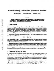
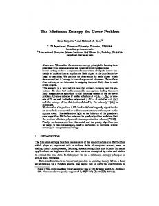
EXAMPLES Synthetic examples The algorithms will be tested in this section. For simplicity, they are called MED (Wiggins’s algorithm) and FMED (minimum entropy with frequency-domain constraints). The logarithmic norm (Table 1) is used in all the cases. The algorithms were tested with the same synthetic data. The seismic trace was generated by convolving a zero-phase 15-60 Hz pass-band wavelet with a reflectivity series. The model (reflectivity) and the synthetic seismic trace are shown in Figures la and lb. The reflectivity and seismic trace spectra are shown in Figures 2a and 2b. The MED algorithm was run with a 200 ms filter. The MED output after 10 iterations is shown in Figure lc. Since there is only one

Another way to write equation (21) is (21) The upper index n indicates the iteration number and Hk is a zero-phase, stop-band digital filter with cut-off frequencies and The filter removes the mid-band samples of Bk that are replaced by the known midband samples of Equation (21) can be transformed back to time and an equivalent formulation of the problem is found t

(22)

where ht is the impulsive response of the stop-band filter Hk. The LP formulation In the LP method the objective function to be minimized is (23) The minimization of equation (23) is carried out under the constraints given by equation (14). In Levy and Fullagar (1981), they deal with the problem by splitting the constraints into real and imaginary parts:

FIG. 1. Shown in successive traces: (a) reflectivity, (b) band-limited reflectivity, (c) MED output, and (d) minimum entropy with frequency domain constraints (FMED) output.

942

Sacchi et al.

nonzero midband (15-60 Hz) to be inverted, the MED filter cannot estimate the reflectivity series. Obviously, the chosen synthetic wavelet can never be completely inverted because of its band-limited nature. Note that the FMED algorithm is not only effective for reconstructing the high frequencies, but the low-frequency signature of the spectrum is also recovered (see Figures 1d and 2d). An analysis of the convergence of each algorithm when a band-limited signal is used is shown in Figure 3. After a few iterations, the FMED algorithm reaches a useful maximum. Even after many iterations, the MED does not lead to a useful maximum; actually the maximum reached corresponds to a degenerated solution. To illustrate the behavior of the algorithms under noisy conditions, noise has been added to the synthetic trace with a signal-to-noise ratio of 14 dB (Figure 4b). The MED and FMED outputs are shown in Figures 4c and 4d. Their amplitude spectra are shown in Figure 5. In each iteration, the FMED suppresses the high and low bands where the noise contribution is dominant, and estimates new low and high frequencies from those in the midband.

use this algorithm. The second approach (LP) uses the nonzero frequency band as a constraint and attempts to find a reflectivity model that consists of isolated spikes. The LP approach has been described in a previous section. In Figure 6a, the reflectivity model is shown. In Figure 6b the same model is shown after being filtered with a zerophase operator with f L = 20 Hz and f H = 90 Hz. In Figures 6c, 6d, and 6e the outputs for the FMED, AR, and

Comparison with the LP and AR methods In this section we wish to compare the FMED with the AR modeling technique (Walker and Ulrych, 1983) and the LP reconstruction algorithm (Levy and Fullagar, 1981; Oldenburg et al., 1983). Briefly, it can be said that the AR modeling technique fits a complex autoregressive model to the nonzero band and extrapolates the low and high frequencies by linear prediction. A more sophisticated version of the algorithm applies a gap filling technique that improves the reconstruction of the low-frequency components. This is the way we are going to

FIG. 2. Graphs (a, b, c, d) are the amplitude spectra of the time series of Figure 1.

FIG. 3. Entropy norm versus iterations for the noise-free example.

FIG. 4. Shown in successive traces: (a) reflectivity, (b) band-limited reflectivity plus random noise (SNR = 14 dB), (c) MED deconvolution, and (d) minimum entropy with frequency-domain constraints (FMED) output.


94

LP methods are shown. In the AR reconstruction, the autoregressive operator was computed using a complex Burg algorithm (Walker and Ulrych, 1983). The length of the operator is 0.3( kH - kL ) samples. In Figure 7 we show the spectrum of the reflectivity (7a), the spectrum of the bandlimited reflectivity (7b), and in successive traces, the spectra of the FMED, AR, and LP full-band reflectivity estimates. The reflectivity spectra are reconstructed with different levels of accuracy by all of the techniques. In the AR and FMED case, it is clear that the low-frequency portion of the spectrum is well recovered. However, both methods attempt to overestimate the high-frequency portion of the spectra. Strictly speaking, the AR does not produce much better results than the FMED. Actually, the computational cost involved in the LP is much more expensive than the computational cost of the FMED. In the LP case, the linear programming problem is solved. The latter goal is achieved with a routine based on the simplex method (Levy and Fullagar, 1981). On the other hand, the FMED algorithm needs only two FFTs per iteration. Thus we believe that FMED is worth considering when we seek a fast and easy way to process band-limited data. It is difficult to say which is the best method to invert band-limited data. The block interpretation of several techniques allows us to explore the model space, as well as to have an efficient way to assess the main features of the model manifested in the output of each inversion. Real data In many real applications, it is not necessary to obtain a full-band reflectivity, it is enough to simply extend the band only 10 or 20 Hz to increase resolution. That is the case we are going to present. In the CDPs of Figure 8a, the zone of interest is located at 1250 ms. A zero-phase deconvolution

FIG. 5. Graphs (a, b, c, d) are the amplitude spectra of the time series in Figure 4.

FIG. 6. Comparison of the FMED algorithm with the AR LP methods. (a) Reflectivity, (b) band-limited reflectivity FMED, (d) AR, and (e) LP.

FIG. 7. Amplitude spectra of the traces shown in Figure Reflectivity, (b) band-limited reflectivity, (c) FMED, (d) and (e) LP.

Sacchi et al.

944

was applied to remove the wavelet, producing the mean spectra shown in Figure 9a. The band from 10 to 70 Hz is the constraint of the problem, but instead of extending the high frequencies up to the Nyquist frequency (125 Hz), the band was extended from only 70 to 90 Hz. The low-frequency band was completely extended. The output is shown in Figure 8b. Note a small splitting of the reflections at 1275 ms. This result was later confirmed with a synthetic seismogram (there is a well at CDP 4640). In Figure 8b the mean spectrum of the extended data is shown. In this application, the reconstruction of only a few samples of the reflectivity spectra has been made to get a reliable model. CONCLUSIONS The minimum entropy algorithm with frequency-domain constraints offers a different way to process band-limited data. We have shown that it is possible to reconstruct a spike-like reflectivity series from a portion of its spectrum. When compared with the original reflectivity series, the reconstructed signal results are similar, even when noise is added to the data. The algorithm is robust under noise conditions. This is because the low- and high-band frequency estimates are calculated from the known midband frequency samples where the signal spectrum is dominant.

The well known LP (Levy and Fullagar, 1981; Oldenburg et al., 1983) and AR (Lines and Clayton, 1977; Walker and Ulrych, 1983) procedures were compared with the algorithm presented. The three methods offer similar results, although the LP seems to estimate high frequencies better than the AR and FMED. We believe that the FMED constitutes an efficient and easy way to perform the inversion of bandlimited data, and we strongly believe the proposed approach provides an unifying thread between Wiggins’s approach and the linear programming method. Finally, the effectiveness of the FMED was tested with field data. In this example, the FMED was used to resolve two close reflections. The result was later verified with a synthetic seismogram computed from a sonic log at the productive level of the well. ACKNOWLEDGMENTS This work was partly supported by the Consejo National de Investigaciones Cientificas y Tecnicas (Argentina). Also, we wish to thank Prof. T. J. Ulrych for supplying the AR and LP codes used in the preparation of the paper. M. D. Sacchi would like to thank Prof. T. J. Ulrych for his useful comments and support.

FIG. 8. Example with real data. (a) Segment of seismic section. The data were preprocessed with a zero-phase deconvolution routine. (b) After recovering the low frequencies and part of the high frequencies with the FMED.


945

FIG. 9. (a) Mean amplitude spectrum of the seismic segment (Figure 8a). (b) Mean amplitude spectrum of the seismic segment after processing with FMED (Figure 8b). REFERENCES De Vries, D., and Berkhout, A. J., 1984, Velocity analysis based on minimum entropy: Geophysics, 49, 2132-2142. Levy, S., and Fullagar, P. K., 1981, Reconstruction of a sparse spike train from a portion of its spectrum and application to high-resolution deconvolution: Geophysics, 46, 1235-1243. Lines, L. R., and Clayton, R. W., 1977, A new approach to Vibroseis deconvolution: Geophys. Prosp., 25, 417-433. Oldenburg, D. W., 1981, A comprehensive solution to the linear deconvolution problem: Geophys. J. Roy. Astr. Soc., 65, 331-357. Oldenburg, D. W., Scheuer, T., and Levy, S., 1983, Recovery of the acoustic impedance from reflection seismograms: Geophysics, 48, 1318-1337.

Parker, R. L., 1977, Understanding inverse theory: Ann. Rev. Earth Planet. Sci., 5, 35-64. Postic, A., Fourmann, J., and Claerbout, J., 1980, Parsimonious deconvolution: Presented at the 50th Ann. Mtg., Soc. Expl. Geophys. Robinson, E. A., and Treitel, S., 1980, Geophysical signal analysis: Prentice-Hall, Inc. Sacchi, M. D., Velis, D. R., and Cominguez, A. H., 1992, A comparative study of two simplicity norms: Geoacta, 19, 181-194. (in Spanish with abstract in English) Walker, C., and Ulrych, T. J., 1983, Autoregressive recovery of acoustic impedance: Geophysics, 48, 1338-1350. Wiggins, R. A., 1978, Minimum entropy deconvolution: Geoexpl., 16, 21-35