ulary in dc to ac inverters which are used in ac motor drives and continuous ac power supplies where the objective is to produce a sinusoidal ac output whose.
Decoupling Control of d and q Current Components in Three-Phase Voltage Source Inverter Mirjana Milosevic Abstract The current control is an important issue in power electronic circuits, particulary in dc to ac inverters which are used in ac motor drives and continuous ac power supplies where the objective is to produce a sinusoidal ac output whose magnitude and frequency can both be controlled. In this paper, the current control of three-phase pulse width modulated voltage source inverter (PWM-VSI) has been implemented in the rotating d,q reference frame. Introduction Three major classes of regulators have been developed over last few decades: hysteresis regulators, linear PI regulators and predictive dead-beat regulators [1]. Although high performance control strategies have been proposed, they still exhibit coupling problems not providing the decoupling of the active and reactive current components (not allowing the independent control of the active and reactive power) [2]. These classes can be further divided into stationary and synchronous d,q reference frame implementations by applying ac machine rotating field theory [3]. The relationship between stationary and synchronous frame controllers is given in [4]. A short review of the available current control techniques for the three-phase systems is presented in [5]. The synchronous frame controller has, also, become the standard solution for current control of PWM rectifiers [6]. The real-time control strategy based on a non-linear state variables feedback approach that decouples the active and reactive line current components allowing the independent control of active and reactive supply power has been proposed in [7]. The decoupling control has been also applied on high speed operation of induction motors where its depends on the accuracy of the stator inductance and the leakage factor [8]. In this paper, the current control of PWM-VSI has been implemented in the rotating (synchronous) d,q reference frame because the synchronous frame controller can eliminate steady state error and has fast transient response by decoupling control. However, synchronous frame controller is more complex then the stationary frame controller and requires transforming of measured stationary frame ac current to rotating frame dc components, and transforming the result of control back to the stationary frame for implementation. Two methods of decoupled current control are explained here: feedforward 1
and feedback decoupling control. Mathematical Model of the Three-Phase VSI The power circuit of three-phase VSI is shown in figure 1. idc Sa
ia
L
R
ib
L
R
ic
L
R
+
Vsa
R1 C
+
Vdc
Sb
+
Vsb
-
V Sc
+
Vsc
Figure 1: VSI power topology The dc and ac side equivalent circuits of the VSI are depicted in figure 2.
[i]abc R1 V
+
vdc -
L
[v]abc
C
+
idc
-
R +
[vs]abc
Figure 2: Equivalent circuit of the VSI Mathematical model of the equivalent circuit is given by:
C
V − vdc dvdc + idc = dt R1
(1)
L
d[i]abc + Ri = ∆[v]abc dt
(2)
ia + i b + i c = 0
where ∆[v]abc = [v]abc − [vs ]abc .
2
(3)
Applying the transformation method from three-phase system (abc) to rotating frame (dq):
·
xd xq
¸
cos w1 t 2 cos(w1 t − 120◦ ) = 3 cos(w1 t + 120◦ )
T xa − sin w1 t − sin(w1 t − 120◦ ) × xb xc − sin(w1 t + 120◦ )
(4)
to the current [i]abc we have: 2 [ia cos w1 t + ib cos(w1 t − 120◦ ) + ic cos(w1 t + 120◦ )] 3
(5)
2 iq = − [ia sin w1 t + ib sin(w1 t − 120◦ ) + ic sin(w1 t + 120◦ )] 3
(6)
id =
and similarly to the voltage [∆v]abc we have:
∆vd =
2 [∆va cos w1 t + ∆vb cos(w1 t − 120◦ ) + ∆vc cos(w1 t + 120◦ )] 3
2 ∆vq = − [∆va sin w1 t + ∆vb sin(w1 t − 120◦ ) + ∆vc sin(w1 t + 120◦ )] 3
(7)
(8)
If we apply the derivative to equation 5:
2 dia dib dic did = [ cos w1 t + cos(w1 t − 120◦ ) + cos(w1 t + 120◦ )]− dt 3 dt dt dt
(9)
2 − w1 [ia sin w1 t + ib sin(w1 t − 120◦ ) + ic sin(w1 t + 120◦ )] 3
From equation 2 we have that: dia 1 R = ∆va − ia dt L L dib 1 R = ∆vb − ib dt L L dic 1 R = ∆vc − ic dt L L 3
(10)
Using equations 5, 6, 7 and 10, equation 9 can be rewritten as : did R 1 = w1 iq − id + ∆vd dt L L
(11)
Similarly, if we apply the derivative to equation 6 we have: R 1 diq = −w1 id − iq + ∆vq dt L L
(12)
Equations 11 and 12 can be transformed in the Laplace domain (s-domain) as:
(sL + R)Id = ∆Vd + w1 LIq
(13)
(sL + R)Iq = ∆Vq − w1 LId
(14)
Multiplying equation 14 with the complex number j and adding to equation 13 we have:
(sL + R)(Id + jIq ) = ∆Vd + j∆Vq + w1 L(Iq − jId )
(15)
which can be rewritten as: → − → − (sL + R + jw1 L) I = ∆ V
(16)
→ − → − where I = Id + jIq and ∆ V = ∆Vd + j∆Vq . The transfer function G(s) of the circuit is given with: → − 1 I G(s) = → − = sL + R + jw L 1 ∆V
4
(17)
Id
Vd
+
sL+R
wL
wL
Iq
+ sL+R
Vq
+
Figure 3: Crosscoupling of the d and q components It can be seen from equation 17 that there is a cross-coupling between the d and q components (because of the jw1 L part) which is also depicted in the figure 3. However, crosscoupling can affect the dynamic performance of the regulator [9]. Therefore, it is very important to decouple the coupling term for better performance. Decoupling Methods In this paper we applied two decoupling methods: feedforward and feedback decoupling method for current control of VSI in rotating d,q frame. 1) Feedforward method Iref +
PI -
V’
Decoupling
dq
V+
abc
+
Switching control
I VSI Vs
dq abc
dq abc
Figure 4: Current control of VSI (feedforward decoupling method) The block diagram of the current control of VSI with feedforward decoupling method is shown in figure 4. The decoupling part from the same figure is given in figure 5 separately, − → where ∆V 0 is the controlled voltage (output of the PI controller employed in active and reactive current control in VSI). In order to have d and q components decoupled we want to define transfer function G1 such that:
5
, V
V
G1(s)
I
G(s)
Figure 5: Feedfoward decoupling
Gdc (s) =
− → 1 I − →0 = sL + R ∆V
(18)
From figure 5 we can calculate: → − → − I = G(s)∆ V
(19)
− → → − ∆ V = G1 (s)∆V 0
(20)
combining these two equations and equation 18 and knowing, also, that G dc (s) = G1 (s)G(s) the transfer function G1 (s) is defined as:
G1 (s) = 1 + j
w1 L sL + R
(21)
2) Feedback method
Iref + -
PI
V’
dq
V+ +
abc
+
Switching control
I VSI Vs
dq abc
Decoupling
dq abc
Figure 6: Current control of VSI (feedback decoupling method) The block diagram of the current control of VSI with feedback decoupling method is shown in figure 6. The decoupling part from the same figure is given in figure 7 separately, − → where ∆V 0 is the controlled voltage (like in the feedforward decoupling method).
6
, V
V
+
G(s)
I
+
G2(s) Figure 7: Feedback decoupling Similarly as in the previous method we have to define the transfer function G2 (s) such that the equation 18 is valid. From figure 7 can be seen that: − → → − → − ∆ V = G2 (s) I + ∆V 0
(22)
Equation 19 is valid here, also. From equation 19 and 22 we have: − → → − (1 − G(s)G2 (s)) I = G(s)∆V 0
(23)
Finally, we have that:
Gdc (s) =
→ − G(s) I − →0 = 1 − G(s)G (s) 2 ∆V
(24)
Combining this equation with equations 18 and 17 it can be seen that decoupling transfer function G2 (s) in the case of feedback method is given with: G2 (s) = jw1 L
7
(25)
Simulation Results The VSI shown in figure 1 has been simulated using both Simulink and PLECS. Simulation results for steady state are presented in figure 8 (feedforward method) and in figure 10 (feedback method). Also, simulation results for the step change in reference current are given in figures 9 and 11 for both methods. The circuit parameters are L=2mH, C =100µF, f =50Hz, V=400V, R1 = 1Ω, Idref = 10A, Iqref = 0A (after 0.01 sec Idref = 15A). Feedforward decoupling (id,iq) 20
15
id,iq
10
5
0
−5
−10
0
0.005
0.01
0.015 time [sec]
0.02
0.025
0.03
Figure 8: d and q current components using feedforward decoupling method Feedforward decoupling method (id, iq) 25
20
15
id,iq
10
5
0
−5
−10
0
0.005
0.01
0.015
0.02
0.025 time[sec]
0.03
0.035
0.04
0.045
0.05
Figure 9: d and q current components using feedforward decoupling method with step change in reference current
8
Feedback decoupling (id,iq) 14
12
10
8
id,iq
6
4
2
0
−2
−4
0
0.005
0.01
0.015 time [sec]
0.02
0.025
0.03
Figure 10: d and q current components using feedback decoupling method
Feedback decoupling method 20
15
id,iq
10
5
0
−5
0
0.005
0.01
0.015
0.02
0.025 time[sec]
0.03
0.035
0.04
0.045
0.05
Figure 11: d and q current components using feedback decoupling method with step change in reference current
9
Comments From equation 21 it can be concluded that when R → 0 the value of the inductance is not necessary to be known and that could be an advantage of the feedforward method, which is not the case with the feedback method where we have to know value of inductance (equation 25). On the other hand, under the same conditions (when R → 0) we have an oscillatory behavior in the feedforward method due to the integration (we have the integrator part 1/s), and we do not have oscillations in the feedback method. It can be seen, as well, in figures 8 and 10.
10
References 1. S. Buso, L. Malesani, P. Mattavelli, ”Comparison of Current Control Techniques for Active Filter Applications”, IEEE Transaction on Industrial Electronics, Vol. 45, No.5, October 1998., pp.722-729 2. J. Choi, S. Sul, ”Fast current controller in three-phase ac/dc boost converter using d-q axis crosscoupling”, IEEE Transaction on Power Electronics, Vol. 13, pp. 179-185, Jan. 1998. 3. Y.Sato, T. Ishiuka, K. Nezu, T.Kataoka, ”A New Control Strategy for Voltage-Type PWM Rectifiers to Realise Zero Steady-State Control Error in Input Current”, IEEE Transaction on Industry Applications, Vol. 34, No.3, pp. 480-486, 1998. 4. D. N. Zmood, D. G. Holmes, ”Stationary Frame Current Regulation of PWM Inverters with Zero Steady State Error”, PESC ’99., pp. 1185 -1190, Vol.2 5. M.P. Kazmierkowski, L. Malesani, ”Current control techniques for threephase voltage-source PWM converters: a survey”, Industrial Electronics, IEEE Transactions on Industrial Electronics, Vol. 45, No. 5, Oct.1998., pp. 691 -703 6. M.P. Kazmierkowski, M. Cichowlas, ”Comparison of current control techniques for PWM rectifiers ”, Proceedings of the 2002 IEEE International Symposium on Industrial Electronics, Vol. 4, pp. 1259 -1263 7. J.R. Espinoza, G. Joos, L. Moran, ”Decoupled control of the active and reactive power in three-phase PWM rectifiers based on non-linear control strategies” PESC ’99., pp. 131 -136, Vol.1 8. J. Jung, K. Nam, ”A dynamic decoupling control scheme for high-speed operation of induction motors”, IEEE Transactions on Industrial Electronics, Vol. 46, No. 1 , Feb. 1999., pp. 100 -110 9. D. N. Zmood, D. G. Holmes,G.H. Bode,”Frequency-domain analysis of threephase linear current regulators”, IEEE Transactions on Industry Applications, Vol. 37, No. 2, March-April 2001., pp. 601 -610
11