Laboratory of Algorithms, Complexity and Logic (LACL), University of Paris-East. {frederic.gava ...... code from Java using a tool call Krakatoa. Third, the ...
Deductive Verification of State-Space Algorithms Fr´ed´eric Gava, Jean Fortin, and Michael Guedj Laboratory of Algorithms, Complexity and Logic (LACL), University of Paris-East {frederic.gava,jean.fortin,michael.guedj}@univ-paris-est.fr
Abstract. As any software, model-checkers are subject to bugs. They can thus report false negatives or validate a model that they should not. Different methods, such as theorem provers or Proof-Carrying Code, have been used to gain more confidence in the results of model-checkers. In this paper, we focus on using a verification condition generator that takes annotated algorithms and ensures their termination and correctness. We study four algorithms (three sequential and one distributed) of state-space construction as a first step towards mechanically-assisted deductive verification of model-checkers. Key words: BSP, Model-checking, Deductive verification, State-space.
1
Introduction
Motivation. Model-checkers (MCs for short) are often used to verify safetycritical systems. The correctness of their answers is thus vital: many MCs produce the answer “yes” or generate a counterexample computation (if a property of the model fails), which forces, in the two cases, to assume that the algorithm and its implementation are both correct. But MCs, like any software are subject to bugs and there exist surprisingly few attempts to prove them correct. Three main reasons can explain this fact [13]: (1) MCs involve complicated logics, algorithms and sophisticated state reduction techniques; (2) because efficiency is essential, MCs are often highly optimised, which implies that they may not be designed to be proved correct; (3) MCs are often updated. But there is a more and more pressing need from the industrial community, as well as from national authorities, to get not just a boolean answer, but also a formal proof — which could be checked by an established tool such as the theorem prover Coq. This is required in Common Criteria certification of computer products at the highest assurance level EAL 7 — http://www.commoncriteriaportal.org/. And hand proofs are not sufficient for EAL 7, mechanical proofs are needed. The author of [18] resumes the problem: Quis custodiet ipsos custodes ? (Who will watch the watchmen? that is, who will verify the verifier?). We want to be able to trust the results of model-checkers with a high degree of confidence. Different solutions for verifying model-checkers. For verifying modelcheckers, different solutions have been proposed. The first one is to prove MCs
inside theorem provers and use the extraction facilities to get pure functional machine-checked programs such as in the works of [20] and [6]. The second and more common approach, in the spirit of Proof-Carrying Code [14] (PCC for short), is to generate a “certificate” during the execution of the MC that can be checked later or on-the-fly by a dedicated tool or a theorem prover. This is the so-called “certifying model-checking” [13]. In this way, users can re-execute the certificate/trace and have some safety guarantees because even if the MC is buggy, its results can be checked by a trustworthy tool. But, any explicit MC may enumerate a very large state-spaces (the famous state-space explosion problem), and mimicking this enumeration with proof rules inside any theorem prover (or with PCCs) would be foolish even if specific techniques and optimisations of the abstract machine of theorem provers [1] are used. Note that this problem does not arise when finding a refutation of the logical formula (the trace is generally short) but when the answer is “yes” since the entire explicit state-space (or at least a symbolic representation) needs to verify the checked properties. In this way, certificate generation could also hamstring both the functionality and the efficiency of the automation that can be built from theorem provers (functional programs can be too memory consuming) and PCC tools (too big certificates) [18]. Only efficient, imperative and distributed programs can override the state-space explosion problem. Another solution, proposed in [22] for a MC call PAT, is to use coding assumptions directly in the source code. They indeed use Spec# and a check of the object invariants (the contracts) is generated. Nevertheless, they cannot completely verify the correctness of PAT and they thus focus on some safety properties (as no overflows, no deadlocks) of the underlying data structures of PAT (which can run on a multi-core architecture) and check if some options may conflict with each other. The proposed solution and outline. Our contribution follows the approach of [22] but by using the “verification condition generator” (VCG for short) WHY [7] and by extending the verification to the correctness of the final result: has the full state-space been well computed without adding unknown states? Since the language of WHY is not immediately executable but a higher-level algorithmic language, we only focus on algorithms. We can thus focus on which formal properties need to be preserved and not be obstructed by problems specific to a particular programming language. Even if most of the bugs in MCs will not be due to wrong algorithms but rather due to subtle errors in the implementation of some complex data structures and bad interactions between these structures and compression aspects, we must first check the algorithms to get an idea of the amount of work necessary to verify a true model-checker. Our goal is then a mechanically-assisted proof that these annotated algorithms terminate and indeed compute the expected finite state-space. This is an interesting first step before verifying MCs themselves: it allows to test if this approach is doable or not. This is also challenging due to the nature of model-checking (critical system) and to the algorithmic complexity. The main
contribution of this paper is to demonstrate the ability of a VCG such as WHY to tackle the wide range of verification issues involved in the proof of correctness of imperative codes of MCs. The remainder of this paper is structured as follows. The VCG WHY is presented in Section 2.1, then the full state-space if formally defined in Section 2.2; we consider also verifying different algorithms formally: three sequential ones (which correspond to those mainly used in explicit MCs; described in Section 2.3; verified in Section 2.4) and one distributed — mainly used in explicit distributed MCs; described in Section 3.3; verified in Section 3.4. The first three are relatively simple to prove correct: it is thus a good basis for correctness of MCs. For the last, we use our own extension of WHY called BSP-WHY [9], which is presented in Section 3.2. Section 4 discusses some related work and finally, Section 5 concludes the paper and gives a brief outlook to future work.
2
Verification of sequential state-space algorithms
We now introduce the VCG WHY, describe how we model the state space, and present the verification of 3 well-known algorithms. The annotated source codes are available at http://lacl.fr/gava/cert-mc.tar.gz. 2.1
Deductive verification of algorithms using WHY
WHY [7] is a framework for the verification of algorithms. Basically, it is composed of two parts: a logical language with an infrastructure to translate it to existing theorem provers; and an intermediate verification programming language called WhyML with a VCG for deductive verification. The logic of WHY is a polymorphic first-order logic with logical declarations: definitions and axioms. The examples of the standard library propose finite sets of data and several operations with their axiomatisation (which can be proved using Coq): a constant empty set; functions add, remove, union, inter, diff, cardinal; a predicate for emptiness, equality, subset, extensionality, etc. In the logical formula, x@ is the notation for the value of x in the pre-state, i.e. at the precondition point and x@label for the value of x at a certain point (marked by a label) of the algorithm. WhyML is a first-order language with an ML flavored syntax and it provides the usual constructs of imperative programming. All symbols from the logic can be used in the algorithms. Mutable data types can be introduced, by means of polymorphic references: a reference r to a value of type σ has type ref σ, is created with the function ref, is accessed with !r, and assigned with r ←e. Algorithms are annotated using pre- and post-conditions, loop invariants, and variants to ensure termination. Verification conditions are computed using a weakest precondition (wp) calculus and then passed to the back-end of Why to be sent to provers. Notice that in WHY, sets are immutable (manipulated only with purely functional routines) and thus only a reference on a set can be modified and assigned to another set.
1 2 3 4 5 6 7 8 9
let normal () = let known = ref ∅ in let todo = ref {s0} in while todo 6= ∅ do let s = pick todo in known←!known ⊕ s; todo←!todo ∪ (succ(s) \ !known) done; !known
1 2 3 4 5 6 7 8 9 10
let main dfs () = let known = ref ∅ in let rec dfs (s:state) : unit = known←!known ⊕ s; let current = ref (succ(s) \ !known) in while current 6= ∅ do let new s = pick current in if (new s 6∈ known) then dfs(new s) done; in dfs(s0); !known
Fig. 1. Sequential WhyML algorithms.
2.2
Definition of the finite state-space
Let us recall that the finite state-space construction problem is computing the explicit graph representation (also known as Kripke structure) of a given model from the implicit one. This graph is constructed by exploring all the states reachable through a successor function succ (which returns a set of states) from an initial state s0 . Generally, during this operation, all the explored states must be kept in memory in order to avoid multiple explorations of a same state. In this paper, all algorithms only compute the state-space, noted StSpace. This is done without loss of generality and it is a trivial extension to compute the full Kripke structure — usually preferred for checking temporal logic formulas. To represent StSpace in the logic of WHY, we used the following axiom contain state space (for consistency, it has been proved in Coq using an inductive definition of the state-space, also available in the source code): 1 2 3
logic s0: state logic succ: state → state set logic StSpace: state set axiom contain state space: ∀ss:state set. StSpace ⊆ ss ↔ (s0 ∈ ss and (∀ s:state. s ∈ ss → s ∈ StSpace → succ(s) ⊆ ss))
i.e. defines which sets can contain the state-space. Now ss is the state-space (ss=StSpace) if and only if, the two following properties holds: (A) ss ⊆ StSpace and (B) StSpace ⊆ ss; that is equality of sets using extensionality. Note that using this first-order definition makes the automatic (mainly SMT) solvers prove more proof obligations than using an inductive definition for the state-space. 2.3
Sequential algorithms for state-space construction
Fig. 1 gives two common algorithms in WhyML using an appropriate syntax for set operations — a “Breadth-first” algorithm is also fully available in the source code but not presented here due to lack of space. All computations in these programs are set operations where a set call known contains all the states that have been processed and would finally contain StSpace. The first one, called “Normal”, corresponds to the usual sequential construction of a state-space —random walk. It involves a set of states todo that is used to hold all the states whose successors have not been constructed yet; each state s from todo is processed in turn (lines 4 − 5) and added to known (line 6) while its successors are added to todo unless they are known already — line 7. The second one is the standard recursive algorithm “Dfs”. At each call of dfs(s), the state s is added (side-effect) to known (line 3) and dfs is then recursively called (lines 5 − 8) for all the successors of s unless they are already known
— which is an optimization since these states would anyway be filtered out later on. Note the use of a conditional (line 8) within this loop: this is due to the fact that during the exploration of the successors of s, known can be increased and thus this prevents the re-exploration of these states Note that the “Normal” algorithm can be made strictly depth-first by choosing the most-recently discovered state (i.e. todo as a stack), and breadth-first by choosing the least-recently discovered state. This has not been studied here. 2.4
Verification of these algorithms
For correctness, the previously presented codes need three properties: (1) they do not fail (no rule of reduction); (2) they indeed compute the state-space; (3) and they terminate. The first property is immediate since the only operation that could fail is pick (where the precondition is “not take any element from an empty set”) and this is assured by the guard of the while loop. Let us now focus on the specification of the above algorithms. Annotations. Fig. 2 gives the full annotated code of the “Dfs” algorithm and “Normal” needs only adding the following invariants in the loop (and final postcondition {result=StSpace}): invariant (1) (known ∪ todo) ⊆ StSpace and (2) (known ∩ todo)=∅ and (3) s0 ∈(known ∪ todo) and (4) (∀ e:state. e ∈known → succ(e) ⊆ (known ∪ todo)) variant |StSpace \ known|
1 2 3 4 5
These four invariants are: (1) known and todo are subsets of StSpace; at the end, (3) and (4) known is a subset of StSpace and has the “same” inductive property; and when todo will be empty, then known contains StSpace — property (B). “Dfs” is more subtle. We need to introduce ghost codes1 , notably a set nofinish (line 3) which has the following rule: each state s in nofinish has been processed by the dfs function but not completely that is, s is in known and not all its direct successors have been processed by dfs — in the loop. It is used in the pre-condition (lines 8-9) and post-condition (lines 31-34) of dfs since not all the direct successors have been processed since it is a depth-first algorithm. Also nofinish is a subset of known since all the time, each state s will be finally completely processed. That also forces us to add this fact in pre- and post- conditions. The post-conditions (1) and (2) are used for (A) and (B). Note the use of nofinish since some states can not be fully processed but nofinish is empty at the end of the computation, ensuring (B). The two post-conditions (5) and (7) say that nofinish is the same before and after dfs (thus empty when s0 is fully processed) but known was able to increase. Now the invariants (lines 18 − 22) of the loop are the following: (1) and (2) as in “Normal”, the set known is a subset of StSpace (current is the set 1
Additional codes not participating in the computation but accessing the program data and allowing the verification of the original code.
1 2 3 4 5 6 7 8 9 10 11 12 13 14 15 16 17 18 19 20 21 22 23 24 25 26 27 28 29 30 31 32 33 34 35 36
let main dfs () = let known = ref ∅ in let nofinish = ref ∅ in (∗ ghost ∗) let rec dfs (s:state) : unit variant |Stspace \ known| = { (1) s ∈StSpace and (2) known ⊆ StSpace and (3) s 6∈ known and (4) s 6∈ nofinish and (5) (∀ e:state. e ∈known→ ¬(e ∈nofinish)→ succ(e) ⊆ known) and (6) nofinish ⊆ known } known←!known ⊕ s; nofinish←!nofinish ⊕ s; let current = ref (succ(s) \ !known) in let ghost diff=ref ∅ in L:while current 6= ∅ do { invariant (1) (known ∪ current) ⊆ StSpace and (2) (∀ e:state. e ∈known→ ¬(e ∈nofinish)→ succ(e) ⊆ known) and (3) succ(s) ⊆ (known ∪ current) and (4) known@L ⊆ known and (5) current@L= (ghost diff ∪ current) and (6) (ghost diff ∩ current)=∅ and (7) nofinish=nofinish@L and (8) nofinish ⊆ known variant |current| } let new s = pick current in ghost diff←!ghost diff ⊕ new s; if (new s 6∈ known) then dfs(new s) done; nofinish←!nofinish s { (1) known ⊆ StSpace and (2) (∀ e:state. e ∈known → ¬(e ∈nofinish) → succ(e) ⊆ known) and (3) s ∈known and (4) s 6∈ nofinish and (5) nofinish=nofinish@ and (6) known@ ⊆ known and (7) nofinish ⊆ known } in dfs(s0); !known {result=StSpace}
Fig. 2. “Dfs” sequential annoted algorithm.
succ(s)−known used in the foreach statement) and known works as StSpace; (3) all the direct successors of s are in known or are currently processed; (4) known can increase; (5 − 6) current works well as an iteration over a set using a ghost set which ensures that no elements are lost during the iteration; (7) nofinish is not modified by the loop but before the loop (and the post-condition ensures that it returns as in the beginning of dfs); (8) nofinish remains a subset of known. Termination. For all the algorithms, termination is ensured by the following variants: |StSpace \ known| and by |current| when an iteration on each state of a set is performed. Each algorithm ensures this first variant at every step using the following properties: – “Normal” only adds a new state s since (known ∩ todo)=∅; – “Dfs” only recursively adds a new state (line 29) since the pre-condition of the function is s 6∈ known (line 8) and the boolean condition of the conditional is new s 6∈ known in the loop for the successors;
Mechanical proof. All the obligations produced by the VCG of WHY are automatically discharged by a combination of automatic provers: CVC3, Z3, Simplify, Alt-Ergo, Yices and Vampire. For each prover, we give a timeout of 10 seconds — otherwise some obligations are not proved. In the following table, for each algorithm, we give the number of generated obligations (column Total) and then how many are discharged by the provers: algo/Solvers Normal Breadth Dfs
Total 11 31 49
Alt-Ergo 2 9 22
Simplify 10 31 48
Z3 11 28 47
CVC3 7 21 40
Yices 3 10 23
Vampire 3 10 26
One could notice that the SMT solvers Simplify and Z3 give the best results. In practice, we mostly used them. Simplify is the faster and Z3 sometime verified some obligations that had not be discharged by Simplify. We also have worked with the provers as black-boxes and we have thus no explanation for this fact. It also took few days for the first author to annotate all the algorithms. Proof obligations are as usual when working with a VCG such as WHY.
3
Verification of a distributed state-space algorithm
Parallelize the construction of the state-space on several machines is a standard method [2, 11]. In this section, we give an example of how to verify a parallel algorithm and show that it is more challenging but feasible. We first present our model of parallel computation called BSP then our own extension of WHY for BSP algorithms and finally the verification of a BSP state-space algorithm. 3.1
The bulk-synchronous parallel (BSP) model
In the BSP model, a computer is a set of uniform processor-memory pairs and a communication network allowing the inter-processor delivery of messages [19, 4]. A BSP program is executed as a sequence of super-steps, each one divided into three successive disjoint phases: each processor only uses its local data to perform sequential computations and to request data transfers to other nodes; the network delivers the requested data; a global synchronisation barrier occurs, making the transferred data available for the next super-step. The BSP model considers communications en masse — as MPI’s collective operations, Message Passing Interface http://www.mpi-forum.org/. This is less flexible than asynchronous messages, but easier to debug and prove since interactions of simultaneous communication actions are typically complex. 3.2
Deductive verification of BSP algorithms
Our tool BSP-WHY extends the syntax of WhyML with BSP primitives (message passing and synchronisation) and definitions of collective operations. BSPWhyML codes are written in a Single Program Multiple Data (SPMD) fashion. We used the WhyML language as a back-end of our own BSP-WhyML language.
Fig. 3. Example of the BSP-WHY’s block decomposition of a BSP code.
In this way, BSP-WhyML programs are transformed into WhyML ones and then the VCG of WHY is used to generated the appropriate conditions for the deductive verification of the BSP algorithm. A special constant nprocs (equal to p the number of processors) and a special variable bsp pid (with range 0, . . . , p−1) were also added to WhyML expressions. A special syntax for BSP annotations is also provided which is simple to use and seems sufficient to express conditions in most practical programs: we add the construct t < i > which denotes the value of a term t at processor id i, and < x > denotes a p-value x (represented by f parray, purely applicative arrays of constant size p) that is a value on each processor as opposed to the simple notation x which means the value of x on the current processor. The transformation of BSP-WhyML codes into WhyML ones is based on the fact that, for each super-step, if we execute sequentially the code for each processor and then perform the simulation of the communications by copying the data, we have the same results as in really truly doing it in parallel. The first step of the transformation is a decomposition of the program into blocks of sequential instructions — Fig. 3. Once that is done for each code block, we create a “for” loop to execute sequentially the block. That is the block is executed p times, once for each processor. Finally, we generate invariants to keep track of which variables are modified: since we are using arrays to represent the variables local to every processor and programs are run in a SPMD fashion, it is necessary to say that we only modify a variable on the current processor and that the rest of the array stays unchanged. Also, when transforming a if or while structure, there is a risk that a global synchronous instruction (a collective operation) might be executed on a processor and not on the other. We generate an assertion to forbid this case, ensuring that the condition associated with the instruction will always be true on every processor at the same time — thus forbidding deadlocks. The details and some examples are available in [9]. The trustworthiness of this tool is discussed in the conclusion. 3.3
BSP state-space construction
Algorithm “Normal” can be easily parallelised using a partition function cpu that returns for each state a processor id, i.e., the processor numbered cpu(s) is the owner of s: logic cpu: state → int axiom cpu range: ∀s:state. 0≤ cpu(s)0 do let tosend = (local successors known todo pastsend) in exchange todo total !known pastsend !tosend done; !known
1 2 3 4 5 6 7 8 9 10 11 12 13 14 15
let local successors (...) = let tosend = ref (init send ∅) in while todo 6= ∅ do let s = pick todo in known←!known ⊕ s; let new states = ref ((succ s) \ !known \ !pastsend) in while new states 6= ∅ do let new s = pick new states in let tgt=cpu(new s) in if tgt=bsp pid then todo←!todo ⊕ new s else tosend←tosend ⊕ new s done done; !tosend
Fig. 4. Parallel (distributed) BSP-WhyML algorithm for state-space construction.
The idea is that each process computes the successors for only the states it owns. This is rendered as the BSP algorithm of Fig. 4. Sets known and todo are still used but become local to each processor and thus provide only a partial view on the ongoing computation. Function local successors computes the successors of the states in todo where each computed state that is not owned by the local processor is recorded in a set tosend together with its owner number. The set pastsend contains all the states that have been sent during the past super-steps — the past exchanges. This prevents returning a state already sent by the processor: this feature is not necessary for correctness and consumes more memory but it is generally more efficient mostly when the state-space contains many cycles. Function exchange is responsible for performing the actual communications: it returns the set of received states that are not yet known locally together with the new value of total — it is essentially the MPI’s alltoall primitive. To ensure termination of the algorithm, we use the additional variable total in which we count the total number of sent states. We have thus not used any complicated methods as the ones presented in [2]. It can be noted that the value of total may be greater than the intended count of states in todo sets. Indeed, it may happen that two processors compute a same state owned by a third processor, in which case two states are exchanged but then only one is kept upon reception. In the worst case, the termination requires one more super-step during which all the processors will process an empty todo, resulting in an empty exchange and thus total = 0 on every processor, yielding the termination. 3.4
Verification of the parallel algorithm
For lack of space, we only present the verification of the parallel part of this algorithm and not the sequential local successors (similar to “Normal” but with many additional invariants on states to send) nor exchange — which is more technical and without really interesting properties and still available in the source code: the exchange procedure is only a permutation of the states that is, from a global point of view, only states in arrays have moved and there is no loss of
states and a state has not magically appeared during the communications. Fig. 5 gives the annotated parallel algorithm. We also use the following predicates: – isproc(i) is defined what is a valid processor’s id that is 0≤ i0 do { invariant S S (1) S() ∪ S() ⊆ StSpace and (2) ( () ∩ ())=∅ and (3) GoodPart() and GoodPartt() and (4) (∀ i,j:int. isproc(i) S → isproc(j) → total = total) and (5) total S ≥ | ()| S and (6) s0 ∈( () ∪ ()) S S S and (7) (∀ e:state. e ∈ () → succ(e) ⊆ ( () ∪ ())) and (8) (∀ e:state. ∀i:int. isproc(i) → e ∈known → succ(e) ⊆ (known ∪ pastsend)) S and (9) () ⊆ StSpace and (10) (∀ e ∈pastsend → cpu(e)6= i) S i:int. isproc(i) → ∀e:state. S S and (11) () ⊆ ( () ∪ ()) S variant pair(total,| S \ (known) |) for lexico order } let tosend=(local successors known todo pastsend) in exchange todo total !known !tosend done; !known S {StSpace= () and GoodPart()}
Fig. 5. Parallel annotated algorithm.
would be sent during the next super-step. At least, one processor cannot received any state during a super-step. We thus need an invariant in the local successors for maintaining the fact that the set known potentially grows with at least the states of todo. We also maintain that if todo is empty then no state would be sent (in local successors) and received, making total equal to 0 — in exchange. Mechanical proof. With some obvious axioms on the above predicates (such S as =∅) so that solvers can handle the predicates, all the produced obligations are automatically discharged by a combination of the solvers. In the following table, for each part of the parallel algorithm, we give the number of obligations and how many are discharged by the provers (some proof obligations require long timeouts e.g. 10 mins): part/Solvers main successor exchange
Total 106 46 24
Alt-Ergo 74 16 20
Simplify 98 42 22
Z3 101 41 23
CVC3 0 24 0
Yices 54 14 16
Vampire 78 32 15
Now the combination of all provers is needed since none of them is able to prove all the obligations. This is certainly due to their different heuristics. We also note that Simplify and Z3 remain the most efficient. Some obligations are hard to follow due to the parallel computations. But reading them carefully, we can find the good annotations. An interesting point is that the first author with the help of an undergraduate student was able to perform the job (annotate this parallel algorithm) in three months. Based on this fact, it seems conceivable that a more seasoned team in formal methods can tackle more substantial algorithms (of model-checking) in a real programming language.
Model Checkers
PCC
treat with a [20, 6]
Proof of correctness
[22] and our work
annotations
VCG
SMT solvers
[?] =
Work we do not know
[13, 15, 23] [12]
[?]
[5]
[21]
Theorem provers
[?]
[3]
Fig. 6. Different ways for proving model-checking algorithms.
4
Related work
Other methods for proving the correctness of model-checkers. Fig. 6 summarises different methods that have been used for verifying MCs where each arrow corresponds to a proof of correctness (using a theorem prover or a PCC approach) and the papers related to the work. The state-space explosion can be a problem for MCs extracted from theorem provers. They are pure functional programs such as the ones of [20, 6]. They certainly would be too slow for big models even if there work on obtaining imperative programs from extracted (pure) functional programs. The “certifying model-checking” is an established research field [15, 23]. But, the performance issue of PCC is discussed in [26] and [16] where the authors present developments (and model-checking benchmarks) of BDDs and tree automata using theorem provers: BDDs are common data-structures used by MCs and tree automata is an approach for having a formal successor function. PCC only focuses on the generation of independently-checkable evidences as the compiled code satisfies a simple behavioural specification such as memory safety; the evidence can then be checked efficiently. Using PCC for state-space is the same as computing it a “second time”. In fact, the drawback of proof certificates is that verification tools have to be instrumented to generate them, and the size of fully expanded proofs may be too large. Authors of [26, 16] conclude that PCCs are here inadequate and we can conclude that MCs themselves need to be proved. It is also the conclusion of [8] where the authors note that “to avoid the inefficiency of fully expansive proof generations, a number of researchers have advocated the verification of decision procedures”. Using annotations in source codes (programs or algorithms) and a VCG has the advantage that realistic and efficient codes (mainly imperative ones) may be verified which could be difficult using theorem provers. And it will not be worth checking all the execution results of the MCs (which can take time) as in the PCC approach because the results will be guaranteed. In our work, we also only use automatic solvers for proving the generated goals of the VCG WHY and thus we do not use any “elaborate” theorem prover such as Coq. The correctness of our results depends on the correctness of (1)
the WHY tool (correct generation of goals) and (2) the results of the solvers. Relying on modules like SMT solvers has the advantage that these tools would certainly be verified in a close future. The work of [12] is a first approach for (1) and the work of [5] is a PCC approach for (2). Moreover, a SMT solver has been proved using a theorem prover [21]. In a close future, we can hope to achieve the same confidence in our codes as the MCs extracted from [20, 6], as well as better performances since our codes are realistic imperative codes — and not functional ones from theorem provers. Finally, we think that using annotations (and a VCG tool) has the advantage of being “easy”. And we can prove the correctness of programs or limit the work to some safety properties if the full correctness is too difficult to obtain. And it extends to parallel programs which is not easy using PCCs or theorem provers. Other various works. There are also interesting examples of verified algorithms on WHY’s web page: Dijkstra shortest path, sorting, Knuth-Morris-Pratt string searching, etc. A mechanically assisted proof using Isabelle of how LTL formulae can be transformed into B¨ uchi automata is presented in [17]. CTL* temporal logic is also available in Coq [24]. All these works are interesting since logical theories may be axiomatised in WHY. Model compilation is one of the numerous techniques to speedup modelchecking: it relies on generating source code (then compiled into machine code) to produce a high-performance implementation of the state-space exploration primitives, mainly the successor function. In [10], authors propose a way to prove the correctness of such an approach. More precisely, they focus on generated LowLevel Virtual Machine (LLVM) code from high-level Petri nets and manually prove that the object computed by its execution is a representation of the compiled model. If such a work can be redone using a theorem prover, we will have a machine-checked successor function which is currently axiomatised in WHY.
5
Conclusion
Model checkers are specialised software, using sophisticated algorithms, whose correctness is vital. In this work, we focus on correctness of well-known sequential algorithms for finite state-space construction (which is the basis for explicit model-checking) and on a distributed one designed by the authors. We annotated the algorithms for finite sets operations (available in Coq) and used the VCG WHY (certifying in Coq [12]) to obtain goals that were entirely checked by automatic solvers. These goals ensure the termination of the algorithms as well as their correctness for any successor function — assumed correct and generating a finite state-space. We thus gained more confidence in the code. We also hope to have convinced the reader that this approach is humanly feasible and applicable to real (parallel or sequential) model-checking algorithms. Future goals are clear. First, adapt this work for true MC algorithms — as those for LTL/CTL* mostly Tarjan/NDFS like algorithms. This is challenging in general but using an appropriate VCG, we believe that a team can “quickly” do
it. Second, we are currently proving algorithms and not real codes. Regarding the code structure, this is not really an issue and translating the resulting proof into a verification tool for true programs should be straightforward, mostly if high level data-structures are used: the WHY framework allows a user to generate WhyML code from Java using a tool call Krakatoa. Third, the successor function (computation of the transitions of the state-space) is currently an abstract function. We think to prove (mechanically) the work of [10] to compensate for this deficiency. Fourth, compressions aspects (symmetry, partial order, etc.) must be studied. The work of [25] which uses the B method could be a good basis. And to finish, the transformation of BSP-WhyML into WhyML is potentially not correct. The second author is working on this. The effort for all these works and thus verifying the whole stack of Fig. 6 is not at all within the reach of a single team. But our guess is that each of these stages is largely feasible. Also, machine-checked MCs would certainly be less efficient than traditional ones. But they could be used in addition when it comes to giving greater confidence in the results. We also believe that another interesting application of a verified tool (such as we are envisioning) would be to serve as a reference implementation that is used to compare the results of an efficient implementation over a set of benchmark problems.
References 1. M. Armand, B. Gr´egoire, A. Spiwack, and L. Th´ery. Extending Coq with imperative features and its application to SAT verification. In M. Kaufmann and L. C. Paulson, editors, Interactive Theorem Proving (ITP), volume 6172 of LNCS, pages 83–98. Springer, 2010. 2. J. Barnat. Distributed Memory LTL Model Checking. PhD thesis, Faculty of Informatics Masaryk University Brno, 2004. 3. B. Barras and B. Werner. Coq in Coq. Technical report, INRIA, 1997. 4. R. H. Bisseling. Parallel scientific computation. A structured approach using BSP and MPI. Oxford University Press, 2004. 5. S. B¨ ohme and T. Weber. Fast LCF-style proof reconstruction for Z3. In M. Kaufmann and L. C. Paulson, editors, Interactive Theorem Proving (ITP), volume 6172 of LNCS, pages 179–194. Springer, 2010. 6. J. Esparza, P. Lammich, R. Neumann, T. Nipkow, A. Schimpf, and J.-G. Smaus. A fully verified executable LTL model checker. In Computer Aided Verification (CAV), 2013. to appear. 7. J.-C. Filliˆ atre. Verifying two lines of C with Why3: an exercise in program verification. In Verified Software: Theories, Tools and Experiments (VSTTE), 2012. 8. J. Ford and N. Shankar. Formal verification of a combination decision procedure. In A. Voronkov, editor, Automated Deduction (CADE), volume 2392 of LNCS, pages 347–362. Springer, 2002. 9. J. Fortin and F. Gava. BSP-WHY: an intermediate language for deductive verification of BSP programs. In High-Level Parallel Programming and applications (HLPP), pages 35–44. ACM, 2010. 10. L. Fronc and F. Pommereau. Towards a certified Petri net model-checker. In H. Yang, editor, Programming Languages and Systems (APLAS), volume 7078 of LNCS, pages 322–336. Springer, 2011.
11. H. Garavel, R. Mateescu, and I. M. Smarandache. Parallel state space construction for model-checking. In M. B. Dwyer, editor, Proceedings of SPIN, volume 2057 of LNCS, pages 217–234. Springer, 2001. 12. P. Herms. Certification of a chain for deductive program verification. In Y. Bertot, editor, 2nd Coq Workshop, satellite of ITP’10, 2010. 13. K. S. Namjoshi. Certifying model checkers. In G. Berry, H. Comon, and A. Finkel, editors, Computer Aided Verification (CAV), volume 2102 of LNCS, pages 2–13. Springer, 2001. 14. G. C. Necula. Proof-carrying code. In Principles of Programming Languages (POPL), pages 106–119. ACM, 1997. 15. D. Peled, A. Pnueli, and L. D. Zuck. From falsification to verification. In R. Hariharan, M. Mukund, and V. Vinay, editors, Foundations of Software Technology and Theoretical Computer Science (FSTTCS), volume 2245 of LNCS, pages 292–304. Springer, 2001. 16. X. Rival and J. Goubault-Larrecq. Experiments with finite tree automata in Coq. In R. J. Boulton and P. B. Jackson, editors, Theorem Proving in Higher Order Logics (TPHOL), volume 2152 of LNCS, pages 362–377. Springer, 2001. 17. A. Schimpf, S. Merz, and J.-G. Smaus. Construction of B¨ uchi Automata for LTL Model Checking Verified in Isabelle/HOL. In S. Berghofer, T. Nipkow, C. Urban, and M. Wenzel, editors, Theorem Proving in Higher Order Logics (TPHOLs), volume 5674 of LNCS. Springer, 2009. 18. N. Shankar. Trust and automation in verification tools. In S. D. Cha, J.-Y. Choi, M. Kim, I. Lee, and M. Viswanathan, editors, Automated Technology for Verification and Analysis (ATVA), volume 5311 of LNCS, pages 4–17. Springer, 2008. 19. D. B. Skillicorn, J. M. D. Hill, and W. F. McColl. Questions and answers about BSP. Scientific Programming, 6(3):249–274, 1997. 20. C. Sprenger. A verified model checker for the modal µ-calculus in Coq. In Tools and Algorithms for Construction and Analysis of Systems (TACAS), volume 1384 of LNCS, pages 167–183. Springer-Verlag, 1998. 21. A. Stump, D. Oe, A. Reynolds, L. Hadarean, and C. Tinelli. SMT proof checking using a logical framework. Formal Methods in System Design, 42(1):91–118, 2013. 22. J. Sun, Y. Liu, and B. Cheng. Model checking a model checker: A code contract combined approach. In J. Song Dong and H. Zhu, editors, Formal Engineering Methods (ICFEM), volume 6447 of LNCS, pages 518–533. Springer, 2010. 23. L. Tan and R. Cleaveland. Evidence-based model checking. In E. Brinksma and K. Guldstrand Larsen, editors, Computer Aided Verification (CAV), volume 2404 of LNCS, pages 455–470. Springer, 2002. 24. M.-H. Tsai and B.-Y. Wang. Formalization of CTL* in calculus of inductive constructions. In M. Okada and I. Satoh, editors, Advances in computer science (ASIAN), volume 4435 of LNCS, pages 316–330. Springer-Verlag, 2007. 25. E. Turner, M. Butler, and M. Leuschel. A refinement-based correctness proof of symmetry reduced model checking. In Abstract State Machines, Alloy, B and Z, LNCS, pages 231–244. Springer, 2010. 26. K. N. Verma, J. Goubault-Larrecq, S. Prasad, and S. Arun-Kumar. Reflecting BDDs in Coq. In J. He and M. Sato, editors, Advances in Computing Science (ASIAN), volume 1961 of LNCS, pages 162–181. Springer, 2000.