it is not fully automatic and requires much user ingenuity and supervision. For this reason ... noNavCnt: Nat alt() nav() ... data source. If either of these failure counters has value 3, the receiver enters ..... (On moving from location s1 back to s0, a ...
Deductive Verification of UML Models in TLPVS? Tamarah Arons1 , Jozef Hooman2,3 , Hillel Kugler1 , Amir Pnueli1 , and Mark van der Zwaag2 1
The John von Neumann Minerva Center for Verification of Reactive Systems, Weizmann Institute of Science, Rehovot, Israel 2 Department of Computer Science, University of Nijmegen, The Netherlands 3 Embedded Systems Institute, Eindhoven, The Netherlands {tamarah.arons, hillel.kugler, amir.pnueli}@weizmann.ac.il {hooman, mbz}@cs.kun.nl
Abstract. In recent years, UML has been applied to the development of reactive safety-critical systems, in which the quality of the developed software is a key factor. In this paper we present an approach for the deductive verification of such systems using the PVS interactive theorem prover. Using a PVS specification of a UML kernel language semantics, we generate a formal representation of the UML model. This representation is then verified using tlpvs, our PVS-based implementation of linear temporal logic and some of its proof rules. We apply our method by verifying two examples, demonstrating the feasibility of our approach on models with unbounded event queues, object creation, and variables of unbounded domain. We define a notion of fairness for UML systems, allowing us to verify both safety and liveness properties. Keywords: Formal Verification, Deductive Verification, PVS, UML, State Machines, Semantics, Temporal Logic
1
Introduction
The Unified Modeling Language (UML) [26] is a flexible, general purpose modeling language that is widely used in a variety of domains. In recent years UML has been applied to the development of reactive safety-critical systems, in which the quality of the developed software is a key factor. In these domains, an executable model and the ability to generate production code from the model is an important advantage [21, 5]. This approach is supported by existing commercial case tools [8, 19, 23], which facilitate the generation of code from a subset of the UML diagrams (typically class diagrams and state machine diagrams) combined with a high level object oriented language or action language. In this paper we present a methodology and tool-set that allow us to verify that various properties hold on a UML model. We take a formal verification ?
This work has been supported by EU-project IST 33522 OMEGA [17], and by the John von Neumann Minerva Center for Verification of Reactive Systems.
approach which enables us to derive a mathematical proof of correctness; in contrast, testing and other validation methods can raise the confidence in the developed system and help in finding bugs, but cannot guarantee correctness. The two prevalent methods for formal verification are model checking and deductive verification. There are obvious advantages to the model-checking techniques, the most important being that it is fully automatic and requires no strong familiarity with the internal details of the design. A very serious limitation of model-checking techniques is the limited size of designs which can be fully automatically verified. The alternative approach based on deductive verification does not suffer from such limitations and, in principle, can be used to verify very big designs provided their structure is based on regular patterns. The main drawback of the deductive approach to reactive system verification (as outlined, for example, in [12]) is that it is not fully automatic and requires much user ingenuity and supervision. For this reason, we developed tlpvs [16], a system for the formal verification of linear temporal logic (LTL) properties built on the PVS [14] verification system. The system provides support for a number of proof rules. Special attention has been paid to the verification of systems with an unbounded number of processes, and our rules are robust for such systems. This means that tlpvs can be used in systems with dynamic object creation. Like other formal verification systems, tlpvs depends on a notion of fairness for the verification of liveness properties. Intuitively, fairness is a means of restricting to the set of “reasonable” runs. To the best of our knowledge, no formulation of fairness requirements appears in the UML literature. In this paper we propose a definition, and illustrate its use. The UML diagrams that we consider in this work are class diagrams and state machine diagrams. This choice is motivated by the fact that these are the diagrams that are considered to form the executable kernel in most approaches and advanced tools. At this stage of our work we avoided adding additional diagrams that may show a different behavioral view of the same aspects and may require us to address issues of consistency, even before addressing the challenges of formal verification which are complex enough in their own right. The UML standard leaves certain semantic issues open and these are implemented differently in various tools and approaches. In order to perform formal verification a precise semantic definition must be taken, our semantic decisions follow [2, 7]. Our deductive verification methodology is, however, more general, and can also support semantic decisions other than the ones we took. The executable kernel subset of the UML mentioned above supports complex features, and our approach treats some of the features that are most difficult for verification: dynamic object creation, active and passive objects, unbounded event queues, synchronous and asynchronous communication and unbounded domain variables. While working to develop a practical formal verification methodology we applied and tested this methodology on two examples, each of which illustrates different features. Eratosthenes’ sieve (prime-sieve) provided an example of dynamic object creation, while a model based on a medium altitude
reconnaissance system (mars) included method calls, and allowed us to check how the methodology scales up in larger systems. The structure of this paper is as follows. In Sect. 2 and 3 we outline the language and semantics we used, and detail the mars example. Section 4 overviews tlpvs, and in Sect. 5 we demonstrate its application to the mars example. Section 6 introduces the prime-sieve example. In Sect. 7 we give our fairness requirements, and show how they can be used to verify response properties in prime-sieve. In Sect. 8 we discuss related work and draw conclusions. The PVS files are available at [24].
2
Kernel Language
In this section we use a fragment of the so-called Medium Altitude Reconnaissance System (mars) to introduce our kernel language. This example is part of a case study provided by the Dutch Aerospace Laboratory (NLR). The system controls the movement of a camera in an airplane; ground survey photographs are taken by the camera during the flight. The position and movement of the camera have to be adjusted to the altitude and speed of the plane.
+rcv Monitor
Receiver
prevOK(): Bool currOK(): Bool
altCnt: Nat navCnt: Nat noAltCnt: Nat noNavCnt: Nat
+busCtrl BusController status(): String
alt() nav() noAlt() noNav() ok() error()
+rcv
AltSource
+rcv NavSource
Fig. 1. Example class diagram.
Here we present a part of the bus manager of the system; the class diagram is given in Fig. 1. For our purposes it suffices to know there is altitude data (alt messages), and there is navigation data (nav messages). In case a data source fails to send data, a time-out is issued. Since we did not model time explicitly for this example, we model these time-outs by failure signals (noAlt, noNav ). The central object in the example is a receiver which processes the incoming data. The system further consists of a controller monitor and a bus controller which we do not present in detail here. The monitor can ask the bus controller for a status report by calling a method of the bus controller. In case of an error the monitor will send the error signal to the receiver in reaction to which the receiver enters the controller error location. The monitor sends the receiver the ok signal if the bus controller indicates that the error situation is resolved. The
task that we concentrate on is the detecting of, and response to, failure of the data sources. For each class the behavior of its objects is defined by means of a state machine and methods (program text) for its so-called primitive operations. Other operations are defined by means of the state machine. A state machine transition is labelled with a trigger event, a guard, and a list of actions (and each of these parts may be empty). A trigger event is either an operation call or a signal. The guard is a boolean expression which can be evaluated locally by the object without side-effects. The action part of a transition is a list of basic actions. We consider the following five basic actions: assign a value or reference to an attribute, create an object and assign a reference to it to an attribute, send a signal to a particular object, call an operation of a particular object and assign a result value to an attribute, return from a call. /rcv!alt
�� ?� � r� � 6
/rcv!noAlt
/rcv!nav
� r�
�� ?� � 6
/rcv!noNav
Fig. 2. State machines for the altitude data source (left) and the navigation data source (right).
Both of the data sources (Fig. 2) have the repetitive nondeterministic choice between sending a data message or a failure message. For example, the action rcv!alt is the emission of an alt signal to the receiver. The receiver (Fig. 3) can accept some failure from the data sources, but if either source fails to send data for three consecutive times, it enters an error state. The receiver recovers from the error state if it receives correct data for at least two consecutive times. Counters (with initial value 0) are used to count consecutively accepted signals of one kind. If the receiver is operational then it counts the number of consecutive failure messages it has accepted from each data source. If either of these failure counters has value 3, the receiver enters the bus error location (since it must run to completion before accepting a new signal, see Sect. 3). In the bus error location, positive acceptances of the data messages are counted.
3
Transition Systems
Intuitively, multiple objects each execute their own state machine concurrently. By interleaving and synchronizing the state machine transitions of the objects in the system we obtain a global transition system representing the system behavior on which we can express properties in temporal logic. Each step of this global transition system corresponds to either the execution of an action by one of
noAlt/noAltCnt:= noAltCnt + 1
�� alt/noAltCnt:= 0 ��
alt/altCnt:= altCnt + 1
�� ��
noAlt/altCnt:= 0
[ noAltCnt = 3 ∨ noNavCnt = 3 ] /
s ? ? �altCnt:= 0; navCnt:= 0 ? ?� � HH � j busError - operational � � � � � [ altCnt ≥ 2 ∧ navCnt ≥ 2 ] / 6 6 6 6 noAltCnt:= 0; noNavCnt:= 0
nav/noNavCnt:= 0 noNav/navCnt:= 0
noNav/noNavCnt:= noNavCnt + 1
ok error
nav/navCnt:= navCnt + 1
� � - controlError � � �
error
Fig. 3. Receiver state machine for the mars example.
the objects in the system, or to the triggering of a state machine transition for one of the objects. In the latter case we distinguish between transitions without a trigger (which are enabled if their guard is satisfied), and signal-triggered transitions. The triggering of a transition with an operation call as trigger is combined with the execution of the transition with the call action into one step of the system. (Note that if the action part of the callee also contains an operation call, this would lead to a cascading sequence of synchronizations. Since this greatly complicates the semantics, we currently do not support an operation call in the action part of a transition with a call trigger.) The interleaving is restricted by the run-to-completion assumption (standard in UML 2.0 [26], see also [21]): when an object has been triggered by a call or a signal, it must become stable before it can accept a new event. An object is stable if, in its current location, it has no outgoing triggerless transitions for which the guard is satisfied; a stable object can only proceed by accepting an event. Thus transitions without a trigger have precedence over triggered transitions. Concurrency can also be restricted by the sharing of control: only an object that has control is allowed to execute. To achieve this, the set of objects is partitioned into activity groups which are centered around active objects: a class can be active or passive, and this leads to active or passive objects. Control is shared within activity groups. During execution the control within a group may shift from one object to another. Control changes when performing a call inside the same group, otherwise an object may only lose control if it is stable. 4 4
This notion of activity groups is comparable to that of threads of control ; an active object corresponds to a thread of control and at most one thread is active in each object. To avoid confusion with, e.g., Java-like threads, we decided to avoid the term “thread” and use “activity group” instead.
Operations are synchronous: a caller is suspended (blocked) until the callee executes the return. Signals are sent asynchronously: the sender may continue immediately and the signal is put in a signal queue at the receiver side. Signals are selected from the queue in order of arrival. The definition of the semantics in PVS is parametrized by the particular types that are to be instantiated by the model that we wish to verify: given that a model provides the names used for classes, attributes, locations, etc., and the set of state machine transitions, this theory defines a labelled transition system which is used as input to the verification in tlpvs as explained below in Sect. 4. For more details of our semantics see [7], which also explains how we model features like inheritance, real-time, and primitive operations, that do not play a role in the examples presented in this paper.
4
A Brief Overview of TLPVS
To reduce the enormous manual effort required to complete deductive proofs, we developed tlpvs, a system which embeds temporal logic and its deductive framework within an existing powerful general-purpose high-order theorem prover, PVS [14]. This system includes a formal PVS specification of the LTL temporal logic based on [12] and a framework for defining systems. A number of rules for proving safety and response properties are included in the system, each one accompanied by a strategy supporting its use. These rules and strategies greatly reduce the routine theorem proving interaction. All proof rules used are defined and proved correct within tlpvs. Using them we eliminate the pen-and-paper application of “known” rules typical in many proofs, and the validity of our final proof rests solely on the correctness of PVS. 4.1
Parameterized Fair Systems
The computational model of parameterized fair systems [16] is used for defining systems in tlpvs. This is a variation of the fair discrete systems of [9] which, in turn, are derived from the model of fair transition systems [12]. A parameterized fair system (pfs) is a tuple S = hV, Θ, ρ, F, J , Ci, where – V is a finite set of typed system variables. We define a state to be a typeconsistent interpretation of V . A (state) predicate is a function which maps states to truth values. A bi-predicate defines a binary relation over states. – Θ is a predicate characterizing the initial states called the initial condition. – ρ(V, V 0 ) is a bi-predicate relating a state to its successors called the transition relation. – F is a non-empty fairness domain which is used to parameterize the fairness requirements of justice and compassion. – J is a justice (weak fairness) requirement. This is a mapping from F to predicates. – C is a compassion (strong fairness) requirement.5 5
We do not use compassion requirements in this paper, and omit them from the explanation. The interested reader is referred to [12, 16].
We define a computation of S to be an infinite sequence of states σ : s0 , s1 , s2 , . . . satisfying the following requirements: – Initiality: s0 is initial, i.e., s0 |= Θ. – Consecution: For each j, the state sj+1 is a successor of the state sj . – Justice: For every t ∈ F there are infinitely many J [t]-states in σ. A typical justice requirement is that continuously enabled transitions are eventually taken. For example, in the mars system we may require that the data sources of Fig. 2 send messages infinitely often. The henceforth operator 2 and the eventually operator 3 are defined as: (σ, j) |= 2p ⇐⇒ for all k ≥ j, (σ, k) |= p, (σ, j) |= 3p ⇐⇒ exists k ≥ j, (σ, k) |= p, where (σ, j) |= p denotes that property p holds at position j in σ. 4.2
Parametrized Fair Systems for UML Models
A pfs is an unlabeled transition system. For this reason, our state data-structure includes, in addition to the state information defined in the kernel language, the label of the last transition that has been taken. We may also want to use auxiliary (history) variables in our proofs. The desired auxiliary information varies according to the system and properties to be verified. The transition relation ρ is derived from the kernel semantics transition relation, and the transition relations for auxiliary variables. Similarly, the initial condition Θ requires that both the kernel semantics state and the auxiliary components satisfy their initial conditions. 4.3
Verifying Safety Properties
Intuitively, safety properties assert that “something bad does not happen.” They are of the form 2a, asserting that predicate a holds in every state that the system may reach. The most frequently used rule for proving safety properties is the basic invariance rule, binv [12]. This rule (Fig. 4) states that if a holds at the initial system state, and is preserved by all transitions, then a is a system invariant. It is the rule we use most often in verifying safety properties. Rule binv is implemented within tlpvs, and is applied using strategy binv. Strategy binv applies the rule, and typically manages to discharge premise B1 automatically. User interaction is then required to prove premise B2. However, the strategy does expand the kernel semantics definitions, labeling the different formulas, and distinguishes subsequent cases according to the kind of transition involved (discarding a signal, locally triggered transition, etc).
Rule binv For predicate a, B1. Θ −→ a B2. a(V ) ∧ ρ(V, V 0 ) −→ a(V 0 ) 2a
Fig. 4. Rule binv (basic invariance)
5
Verification of the MARS Example
In this section we describe how tlpvs was used to verify safety properties in the example of Sect. 2. We would like to verify the following property. Property NoError: If the data sources never send noAlt and noNav messages, the receiver never reaches the bus-error location. This property is not inductive (its holding in the current state does not ensure that it will hold in the next state). As is typically the case in theorem proving, to prove it, it is necessary to prove other, more basic, properties, and to strengthen the invariant. We derive a strengthened invariant: Property NoError0 : If the data sources never send noAlt and noNav messages, then: – The receiver never has noAlt or noNav messages in its signal queue; – The receiver’s noAltCnt and noNavCnt counters remain at zero; – The receiver does not reach the bus-error location. This second property is inductive and can be proved using rule binv. Thereafter it is easy to show that NoError is implied by the strengthened property. Proving premise B1 was done by the binv strategy without user intervention. However, proving premise B2 (the property is invariant over the transition relation) did require user interaction. This invariance must be proved for each of the 26 state machine transitions, as well as for the auxiliary actions such as the discarding of signals. The strategy breaks these transitions into groups according to type (e.g., triggered and untriggered transitions in different groups). Each such branch in the proof is dealt with uniformly, that is, we apply the same set of commands to prove the invariance over all triggered transitions (using the then sequencing strategy of PVS). Some transitions differ from others in their group, and must be dealt with separately. However, the majority are dealt with by a common procedure with no user interaction. The resulting proof was far less interactive than had been anticipated.
6
The Sieve of Eratosthenes
Eratosthenes’ prime sieve algorithm is an ancient algorithm for identifying the prime numbers. The algorithm is inherently unbounded as it can be used to verify the primality of arbitrarily large numbers. We built a UML model of this algorithm, and then verified both the safety property that only primes are identified as prime, and the liveness property that every prime is eventually identified. Despite its simplicity, this example allows us to demonstrate our ability to model and verify object creation and unbounded systems.
� r�
g0
/itsSieve!e(counter) � � � /itsSieve:= new Sieve � � � ? � - g1 � � � � g2 � 6
/counter:= counter + 1
e(x)[prime.divides(x)]
� r�
s0
� e(prime)/itsSieve:= new Sieve � � �
�� ?� s1 � 6
e(x)[not prime.divides(x)]/itsSieve!e(x)
Fig. 5. State machines for the prime-sieve generator (above) and sieves (below).
The objects in the prime-sieve algorithm (Fig. 6) are a single generator and an unbounded number of sieves. Each object has a unique identifier: the generator has identifier 1, sieves are numbered from 2 upwards. The counter of the generator is initialized to two. After creating the first sieve, the sieve sends it all the natural numbers from two upwards (by repeatedly sending and then incrementing the value of its counter). On receiving its first signal, a sieve stores this number as its prime, and creates the next sieve, while taking a transition from location s0 to s1. A sieve which has received and stored a prime and is in location s1 is called looping, while if it is at location s0 it is called non-looping. Subsequent numbers received by a looping sieve are compared to its prime number, prime. Numbers which are not multiples of prime are passed on to the next sieve. Intuitively, a number z which is not a prime will be eliminated when it reaches a looping sieve whose prime is a factor of z. If z is a prime, then no sieve will eliminate it and it will bubble through the system until it reaches a non-looping sieve, which will store z as its prime. 6.1
Primes are Correctly Identified
In this section we outline the proof of the safety property that every number identified as prime by a sieve is truly prime:
Property SievesPrime: The number stored in the prime field of a sieve at location s1 is prime. This property is not inductive and can only be proved once we have proved some additional properties. We need to show that composite (non-prime) numbers are eliminated by the sieves before they reach a non-looping sieve. We note that a composite number n must have some prime factor f < n. This factor must precede n in the sequence of signal queues, until f is itself identified as prime by some sieve i. The number n should then be eliminated when it reaches sieve i (if it wasn’t eliminated before). Our argument that n is removed from the system depends on f not being removed, a property which must also be proved. So, to prove the invariance of SievesPrime we prove that every composite number is preceded by a prime factor (FactorsPrecede), a proof which itself depends on showing that primes are not eliminated (PrimesRemain). In addition, we found it useful to prove some technical system properties such as that all numbers in the queues and sieves are greater than one. These properties simplified our proofs, using binv, of FactorsPrecede and PrimesRemain. Property SievesPrime follows quite simply from FactorsPrecede and is also proved using binv. (The main idea is that when a number reaches a non-looping sieve there are no numbers preceding it in the system, and so it is prime.)
7
Fairness and Liveness
Intuitively, liveness properties assert that under certain conditions a given event will occur. They are generally more difficult to verify than safety properties, and entail the use of the system fairness requirements. They typically require that the user devise well-founded ranking functions, whose values decrease until the desired event occurs. In this section we discuss first our proposed definition of fairness requirements for the UML diagrams under discussion (Sect. 7.1). We then discuss our response rule, dist-rank (Sect. 7.2), and finally demonstrate its use in prime-sieve (Sect. 7.3). 7.1
Fairness Requirements for UML Models
To the best of our knowledge, no formal definition of fairness requirements for UML models appears in the literature. We propose the following definition: For every activity group A, if there is always some transition of an object in A enabled, then A takes transitions infinitely often. More formally: 2(2(∃t : enabled (t, A)) −→ 23(∃u : taken(u, A))), where t and u range over transitions.
Rule dist-rank For pfs S = hV, Θ, ρ, F , J , Ci, Given initial and goal predicates p, q, helpful predicates {ht : t ∈ F}, ranking functions δt : Σ 7→ IN with finite support D1. p
→ q ∨
_
ht
t∈F
D2. ht ∧ ρ D3. ht ∧ ρ D4. ht
_ 0 0 hu → q ∨ ∨ δt > δt ∧ u∈F _ ^ For t ∈ F 0 0 0 0 (δu ≥ δu ∨ δd > δd ∧ δd > δu ) → q ∨ d∈F u∈F → ¬J [t] 0
h0t
2(p −→ 3q)
Fig. 6. Rule dist-rank
Observe that fairness is not defined on the level of objects, but on activity groups (although this coincides if all objects are active). Moreover, it is not required that every transition that is continuously enabled be taken, or that the same transition remain continuously enabled – it is sufficient to take any transition currently enabled for the activity group. This is motivated by the observation that switching control between objects in an activity group may cause transitions to become disabled. 7.2
Verifying Response Properties in Unbounded Systems
Object creation complicates verification in that it is not known, a priori, how many objects will participate in a run. Devising appropriate ranking functions is complicated in such systems. We have developed a new rule, dist-rank, which is particularly suited to unbounded systems [16]. A derivation of the well rule [20], dist-rank allows us to distribute a ranking function over a potentially unbounded number of objects in the system. Rule dist-rank (Fig. 6) traces the progress of a computation from an arbitrary p-state to an unavoidable q-state. Intuitively, a well-founded ranking function δ is distributed over the fairness domain. We show that until a q-state is found, δ decreases monotonically. The well-foundedness of δ then assures us that a q-state is eventually encountered. With each helpful predicate ht of the rule we associate the justice requirement J [t]. Intuitively, the helpful predicate defines a set of states in which a just transition is enabled. When this just transition is taken, and ceases to be helpful, the rank decreases. Thus, the helpful set indicates a transition it would be “helpful” to take in order to decrease the rank. Premise D2 ensures that the application of a transition to a state satisfying predicate ht will cause the rank for fairness domain element t to decrease. When
an element decreases, other elements are allowed to increase providing that their new values are strictly smaller than the old value of a decreasing element (D3). The net result is a reduction in the total system rank [16]. As long as the rank does not decrease ht will continue to hold and J [t] will not (D4). Since the system is just J [t] must hold eventually (Sect. 4.1) and so the rank must eventually decrease. Due to the well-foundedness of the ranking functions, the rank cannot decrease infinitely often. Thus, we cannot have an infinite fair computation which avoids reaching a q-state. The well-foundedness of the ranking function depends on it always having finite support. That is, it must be shown that only a finite number of fairness domain elements can have a positive rank at any point. 7.3
Verifying Response in the Sieve Example
In this section we demonstrate how the dist-rank rule can be used to verify that every prime number is eventually found (meaning, it is stored in the prime field of a looping sieve.) Property PrimesFound: ∀z : 2(prime(z) −→ 3(found(z))) We first define the system fairness requirements. In prime-sieve, every object is in its own activity group. The generator always has some transition enabled, and thus the requirement is that eventually it takes a step. A sieve has a transition enabled if its message queue is non-empty. In this case, the requirement is that a transition eventually be taken. Whereas the generator changes location when it takes a step, a looping sieve remains at s1. A change in location can therefore not be used as an indication that a transition was taken. Instead we use an auxiliary boolean flag variable which changes value every time a sieve at location s1 takes a transition. We define the fairness domain as the tuple [loc, pid, flag], where loc is the object location, pid is the object identifier, and flag is an auxiliary variable. The justice conditions then state, intuitively, that the generator changes location infinitely often, and that a sieve with non-empty signal queue will either change location or change its flag variable. We now define a ranking function. We first define a “rank” for objects, and then use this to define ranks for fairness domain elements. We ensure that the rank of the generator decreases with time by making it inversely dependent on the value of the generator counter. It is defined as 2z − counter + 1. For sieve i ≤ z with a non-empty signal queue with value h ≤ z at its head, the rank is calculated as 2z −h−i+1. Since the numbers in the signal queues are monotonically increasing, the rank of the sieve decreases as it processes queue elements. A sieve with an empty signal queue is assigned rank 0. Therefore, when an element is pushed onto sieve i’s empty signal queue, the rank of sieve i increases. The rank of sieve i − 1 will, however, decrease (its signal queue is either empty or has a larger value at its head). To ensure that the new rank of
sieve i is smaller than the old rank of sieve i − 1 (as required by premise D3 of dist-rank), we subtract the object (sieve) identifier from the rank. We have now defined ranks for objects. The fairness domain element d is given the rank of object d.pid, provided the object d.loc is no larger than the current location of d.pid (where g0 < g1 < g2, s0 < s1). As the sieve progresses to location s1 the rank of its various domain elements are set to zero. The number of domain elements with positive rank can thus be viewed as a counter of sorts, decreasing as the sieve approaches location s1. (On moving from location s1 back to s0, a new, lower, rank is allocated to relevant fairness domain elements.) Finite support is guaranteed by defining the rank of a sieve i to be zero if h > z or i > z. It is easy to see that in both cases the activity of the sieve is no longer of interest for verifying the primality of z: if h > z then z must already have passed through the sieve, or have been eliminated. The prime number of a looping sieve is never smaller than the sieve’s identifier, and so for i > z, sieve i’s prime cannot be a factor of z. A transition of the generator is helpful if it is enabled, and the generator counter is less than z. Once z has been generated, the sieve transitions become helpful. A transition of sieve i is helpful if it is enabled and z is in queue i. Having defined the necessary components, and some auxiliary properties (such as that the values in the signal queues are monotonically increasing) we are able to use tlpvs to verify PrimesFound. This property is non-trivial to prove, and its verification took over one person week. However, we regard the fact that it was tractable at all as an indicator of the appropriateness of tlpvs, and the dist-rank rule in particular, to the verification of UML models. The rule dist-rank is implemented in tlpvs together with a strategy for applying it. In addition, many generic theories and strategies of tlpvs proved very useful. For example, a theory of list properties was used when reasoning about messages in the signal queues, and much use was made of pre-existing simplification strategies.
8
Related Work and Conclusions
In this paper we have presented a methodology for the deductive verification of UML models, and demonstrated it on two examples. We present a new definition of fairness for such models. Future work includes the extension of the methodology to features not yet covered (such as orthogonal states) and timed systems. Much work has been done on formal semantics of UML models (e.g., [18, 6]). A two-dimensional propositional linear temporal logic is used to define the semantics of real-time UML behavior [22]. A proof system using PVS is presented, but verification results were not reported. In contrast, we use transition systems to define the UML semantics, and standard LTL for verification. In [25] an axiom-based definition of UML semantics is given, along with a PVS-based verification environment (PrUDE). The authors demonstrate how simple safety properties can be specified and proved. However, it appears that the system does
not include a formal specification of a verification logic (such as LTL) and its proof rules, which we believe are necessary for the specification and verification of more complex properties. For more details on various semantics efforts and a comparison to our work see [2, 7]. Model-checking has been applied to the verification of UML models in [15, 10, 4]. Apart from the state explosion problem which limits the size of the models that can be verified, these techniques can be applied directly only to finite models. Thus features like object creation, unbounded event queues and unbounded domain variables cannot be treated in a straightforward way. To overcome these limitations, [1] presents a symbolic analysis technique which can be tuned to give a finite, possibly inexact representation of the unbounded event queues. A natural class of protocols for which this representation is both finite and exact is studied. In [3] the symmetry-based technique of query reduction and the abstraction technique data-type reduction are applied in the verification of UML models. In [13] the IF tool-box is used for verifying UML models which have been mapped to communicating extended timed automata. In contrast, our deductive approach allows us to verify models directly with unbounded queues and variables and object creation. There is a trade-off here between the added user-interaction in deductive proofs and the need to devise, and work with, specialized methods for model-checking unbounded systems. Our work was done as part of the EU project Omega [17]. According to the Omega approach, users construct UML models using existing industrial case tools. An XMI representation of the model is then used as input to verification tools constructed by the academic partners of the consortium. Some automated preprocessing may be applied at this level, e.g., the flattening of state machines, and subsequently the representation of the model is translated to a representation of the model in PVS by the uml2pvs tool [11]. Future work in the Omega project considers the extension of the uml2pvs tool to translate OCL constraints to PVS.
References 1. W. Damm and B. Jonsson. Eliminating queues from RT UML model representations. In Proc. FTRTFT’02, volume 2469 of LNCS, pages 375–393. Springer, 2002. 2. W. Damm, B. Josko, A. Pnueli, and A. Votintseva. Understanding UML: A formal semantics of concurrency and communication in Real-Time UML. In Proc. 1st Int. Conf. Formal Methods for Components and Objects (FMCO 2002), volume 2852 of LNCS, pages 71–98. Springer, 2003. 3. W. Damm and B. Westphal. Live and let die: LSC-based verification of UMLmodels. In Proc. 1st Int. Conf. Formal Methods for Components and Objects (FMCO 2002), volume 2852 of LNCS, pages 99–135. Springer, 2003. 4. A. David, O. Moller, and W. Yi. Formal verification of UML statecharts with real-time extensions. In Proc. 5th Int. Conf. Fundamental Approaches to Software Engineering (FASE 2002), volume 2306 of LNCS. Springer, 2002. 5. D. Harel and E. Gery. Executable object modeling with statecharts. Computer, July 1997. Also in Proc. 18th Int. Conf. Soft. Eng., Berlin, IEEE Press, 1996.
6. D. Harel and O. Kupferman. On object systems and behavioral inheritance. IEEE Trans. Software Engineering, 28(9):889–903, 2002. 7. J. Hooman and M. B. van der Zwaag. A semantics of communicating reactive objects with timing. Technical report, EU project IST 33522 OMEGA, 2004. Available at http://www-omega.imag.fr. 8. Rhapsody. I-Logix, Inc., products web page. http://www.ilogix.com/products/. 9. Y. Kesten and A. Pnueli. Verification by augmented finitary abstraction. Inf. and Comp., 163:203–243, 2000. 10. A. Knapp, S. Merz, and C. Rauh. Model checking – timed UML state machines and collaborations. In Proc. FTRTFT’02, volume 2469 of LNCS. Springer, 2002. 11. M. Kyas, H. Fecher, F.S. de Boer, J. Jacob, M.B. van der Zwaag, J. Hooman, T. Arons, and H. Kugler. Formalizing UML models and OCL constraints in PVS. In Semantic Foundations of Engineering Design Languages (SFEDL 2004), Electronic Notes in Theoretical Computer Science. Elsevier, 2004. To appear. 12. Z. Manna and A. Pnueli. Temporal Verification of Reactive Systems: Safety. Springer, New York, 1995. 13. I. Ober, S. Graf, and I. Ober. Validation of UML models via a mapping to communicating extended timed automata. In Proc. 11th Int. SPIN Workshop on Model Checking of Software (SPIN’04), volume 2989 of LNCS. Springer, 2004. 14. S. Owre, N. Shankar, J.M. Rushby, and D.W.J. Stringer-Calvert. PVS System Guide. Menlo Park, CA, November 2001. 15. I. P. Paltor and J. Lilius. vUML: A tool for verifying UML models. In Proc. of the 14th IEEE Int. Conf. on Automated Software Engineering (ASE’99). IEEE, 1999. 16. A. Pnueli and T. Arons. TLPVS: A PVS-based LTL verification system. In Verification: Theory and Practice, pages 598–623. Springer, 2003. 17. OMEGA. EU project IST 33522 (Correct Development of Real-Time Embedded systems). Homepage. http://www-omega.imag.fr/. 18. G. Reggio, E. Astesiano, C. Choppy, and H. Hussmann. Analysing UML active classes and associated state machines – A lightweight formal approach. In T. Maibaum, editor, Proc. Fundamental Approaches to Software Engineering (FASE 2000), volume 1783 of LNCS. Springer, 2000. 19. Rational Rose Technical Developer. Rational, Inc., web page. http://www306.ibm.com/software/awdtools/developer/technical/. 20. E. Sedletsky, A. Pnueli, and M. Ben-Ari. Formal verification of the Ricart-Agrawala algorithm. In FST TCS 2000: Foundations of Software Technology and Theoretical Computer Science, volume 1974 of LNCS, pages 325–335. Springer, 2000. 21. B. Selic, G. Gullekson, and P. Ward. Real-Time Object-Oriented Modeling. John Wiley & Sons, New York, 1994. 22. S. Shankar and S. Asa. Formal semantics of UML with real-time constructs. In Proc. 6th Inf. Conf. on the Unified Modeling Language (UML’03), volume 2863 of LNCS, pages 60–75. Springer, 2003. 23. Telelogic TAU. Telelogic, Inc. http://www.telelogic.com/products/tau/. 24. TLPVS. Homepage. http://www.wisdom.weizmann.ac.il/˜verify/tlpvs. 25. I. Traore, D. B. Aredo, and H. Ye. An integrated framework for formal development of open distributed systems. In Proc. of ACM Symposium on Applied Computing, (ACM SAC2003), 2003. 26. UML. Documentation of the Unified Modeling Language. Available from the Object Management Group (OMG), http://www.omg.org.