formance of our previous visual tracker named Deep Con- volutional Particle Filter (DCPF) [10]. Briefly, DCPF uses multiple particles as inputs to VGG-Net [2].
DEEP CONVOLUTIONAL PARTICLE FILTER WITH ADAPTIVE CORRELATION MAPS FOR VISUAL TRACKING Reza Jalil Mozhdehi, Yevgeniy Reznichenko, Abubakar Siddique and Henry Medeiros {reza.jalilmozhdehi, yevgeniy.reznichenko, abubakar.siddique and henry.medeiros}@marquette.edu Electrical and Computer Engineering Department, Marquette University, Milwaukee, WI, USA ABSTRACT The robustness of the visual trackers based on the correlation maps generated from convolutional neural networks can be substantially improved if these maps are used to employed in conjunction with a particle filter. In this article, we present a particle filter that estimates the target size as well as the target position and that utilizes a new adaptive correlation filter to account for potential errors in the model generation. Thus, instead of generating one model which is highly dependent on the estimated target position and size, we generate a variable number of target models based on high likelihood particles, which increases in challenging situations and decreases in less complex scenarios. Experimental results on the Visual Tracker Benchmark v1.0 demonstrate that our proposed framework significantly outperforms state-of-theart methods. Index Terms— Particle Filter, Target Model, Correlation Map, Deep Convolutional Neural Network, Visual Tracking 1. INTRODUCTION One important aspect of visual target tracking is to accurately determine the target position as well as its size. Particle filters have been employed in visual tracking for years because of their ability to perform these tasks robustly [1]. Recently, deep convolutional neural networks have been used to produce highly discriminative target features [2]. Trackers such as HCFT [3], which employ convolutional features in conjunction with correlation filters have shown better visual tracking performance than traditional trackers such as MEEM [4], KCF [5], Struck [6], SCM [7] and TLD [8]. Despite the substantial performance gains obtained in recent years by the aforementioned CNN-correlation methods, their main disadvantage is their inability to vary the size of the target bounding box [9]. By combining CNN-based correlation maps with particle filters, we can overcome this limitation and improve overall tracking accuracy and robustness. We propose two new mechanisms to improve the performance of our previous visual tracker named Deep Convolutional Particle Filter (DCPF) [10]. Briefly, DCPF uses
multiple particles as inputs to VGG-Net [2]. For each particle, it then applies the correlation filter used in HCFT on the extracted hierarchical convolutional features to construct the correlation map. The target position at the current frame is calculated based on the response of the correlation maps. However, similar to HCFT, DCPF tracks a bounding box of fixed size. Another limitation of DCPF and other trackers based on conventional correlation filters is the fact that they generate only one target model. Thus, errors in calculating the final target state cause the target model to be incorrectly updated. In our new visual tracker named DCPF2, we address the first limitation by extending DCPF’s particle filter to estimate the target size. In addition, we employ an adaptive correlation filter, which produces a variable number of target models based on the number of high-likelihood particles have been generated in the previous frame. In frames when the target can be easily tracked, this number is low because the best particle has a high likelihood and fewer particles have similar likelihoods. Conversely, in challenging situations, the target is less similar to the model and hence the likelihood of most particles decreases and the particle weight distribution becomes less centralized. We used the Visual Tracker Benchmark v1.0 [11] to evaluate the performance of the proposed tracker and showed that it performs favorably with respect to other state-of-the-art methods. 2. PROPOSED ALGORITHM In this section, we first explain how our particle filter estimates the target size and its position. Then, our adaptive correction filter is discussed. Fig. 1 shows the proposed approach. 2.1. Particle Filter to Estimate the Target Bounding Box Let the target position and size be represented by � �T zt = ut , vt , ht , wt ,
(1)
where ut and vt are the locations of the target on the horizontal and vertical image axes at frame t, and ht and wt are its
Current Frame, Previous Position & Target Size
Patch 1
Deep CNN + Correlation Filter with Model 1
Correlation Filter for the Next Frame Final Target Size &Position
Patch 1
Model Best Particle
Patch 2 Deep CNN + Correlation Filter with Model 1
Generate Particles
Model 1
Patch 2
Model
Deep CNN
HighLikelihood Particle 2
Sample Patches
Patch N
Deep CNN + Correlation Filter with Model 1
Model 2
Model
Patch HighLikelihood Particle
Model
Correlation Maps
New Patches
Fig. 1. Overview of our proposed tracker. width and height. The target state is given by � �T xt = zt , z˙t ,
(2)
where z˙t is the velocity of zt . The tracker employs a linear motion model to predict the current state of the target x ˆt based on the previous target state xt−1 . The predicted target state is given by x ˆt = Axt−1 , (3) where A is a standard constant velocity process matrix. Then, � �T particles x(i) = z (i) , z˙ (i) are generated by adding samples η (i) ∈ R8 drawn from a zero-mean normal distribution. That is, (i) xt = x ˆt + η (i) , (4) where i = 1, ..., N and N is the number of the particles. In order to limit the number of particles needed, rather than drawing η (i) directly from an eight-dimensional distribution, we draw its samples individually, and change its height and width simultaneously using the same sample (i.e., we change the target scale but not its aspect ratio). In the next step, z (i) are used to sample different patches from the frame t. Each patch is then fed into the CNN to (i) calculate its convolutional feature map. Let fl,d ∈ RM ×Q be the convolutional feature map, where M , Q are the width and height of the map, l is the convolutional layer and d is the number of the channels for that layer d = 1, ..., D. Then, its (j)(i) correlation response map Rl ∈ RM ×Q is given by (j)(i)
Rl
D X (j) (i) = F−1 ( Cl,d f¯l,d ), d=1
(5)
where F represents the inverse Fourier transform [3], j = 1, ..., Kt−1 illustrates the number of models generated in the (j) previous frame t − 1, Cl,d represents channel d of layer l of the correlation filter of the model j, the bar represents complex conjugation and is the Hadamard product. The final correlation response map R∗(j)(i) for the particle i and the model j is calculated based on a weighted sum of the maps for all the CNN layers as proposed in [3]. The likelihood or weight of each correlation response map is calculated by ω (j)(i) =
Q M X X
∗(j)(i)
R(m,q) ,
(6)
m=1 q=1 ∗(j)(i)
where R(m,q) refers to the element of the final correlation response map on row m and column q. In total, we have N × Kt−1 weights. The intuition behind this choice is that feature maps that correspond to the target tend to show substantially higher correlation values than background patches [12]. We then find the maximum weight ωmax overall all the particles and models ωmax = max ω (i,j) . (7) j,i
Let the indexes corresponding to ωmax be i = i∗ (the best particle) and j = j ∗ (the best model). Then, the final target size ∗ ∗ is given by h(i ) and w(i ) . That is, the i∗ -th patch with di∗ ∗ mensions h(i ) and w(i ) is the most similar to the best model ∗ ∗ ∗ C (j ) . Additionally, let R∗(j )(i ) be the correlation response map associated with ωmax , its peak is located at ∗(j ∗ )(i∗ )
[δu , δv ] = max R(m,q) m,q
,
(8)
where m = 1, ..., M and q = 1, ..., Q. The final target position is then calculated by shifting the best particle towards the peak of its correlation map [˜ u, v˜] = [u(i ∗
∗
)
+ δu , v (i
∗
)
+ δv ],
(9)
∗
where u(i ) and v (i ) correspond to the position of the best particle. Thus, the target state at the frame t is � ∗ �T xt = z ∗ , z˙ (i ) , where z˙ (i
∗
)
(10)
is the velocity of the best particle and � ∗ ∗ �T z∗ = u ˜, v˜, h(i ) , w(i ) .
(11)
Algorithm 1 summarizes our method to estimate the target state. Algorithm 1 Calculate the current target state Input: Current frame, correlation filters C (j) , j = 1, . . . , Kt−1 generated in the previous frame, previous target state xt−1 Output: Current target state xt , maximum weight ωmax , N particles x(i) , N × Kt−1 correlation response maps R∗(j)(i) and their weights ω (j)(i) 1: Generate N particles around the predicted target state x ˆt according to Eqs. 1 to 4 2: for Each particle x(i) do 3: for Each of the Kt−1 correlation filters C (j) do 4: Generate the Kt−1 correlation response maps R∗(j)(i) according to Eq. 5 5: Compute the weight ω (j)(i) based on Eq. 6 6: end for 7: end for 8: Determine the best particle using Eq. 8 9: Update the target state xt according to Eqs. 9 to 11
Algorithm 2 Adaptive Correlation Filter Input: Current frame, maximum weight ωmax , N particles x(i) , their N × Kt−1 correlation response maps R∗(j)(i) and weights ω (j)(i) Output: Kt -model correlation filter C (j) to be used in the next frame j 1: for Each weight ωi do 2: if Eq. 12 is true then (s) 3: Generate a high-likelihood particle zhigh according to Eq. 13 4: end if 5: end for (s) 6: for Each particle zhigh do 7: 8:
(s)
Calculate its correlation filter Cl,d end for
where s = 1, ..., Kt and Kt is the number of the highlikelihood particles. We then generate a patch from frame t for each of the Kt high-likelihood particles. In the next step, these patches are fed into the CNN to extract Kt convolu(s) tional feature maps, and a new correlation filter Cl,d is then generated for each of the Kt high likelihood particles. The generated models are used in frame t + 1 to be compared with the convolutional features generated by each particle. Alg. 2 summarizes our adaptive correlation filter procedure. The comparison between the best model with the most accurate target size and position generates more accurate correlation maps. As previously mentioned, by varying the number of models Kt with the number of high likelihood particles, we are able to maintain a larger number of tentative models in challenging scenarios such as in the presence of illumination variation, motion blur, or partial occlusion due to the wider distribution of the particle weights under these conditions. 3. RESULTS AND DISCUSSION
2.2. Adaptive Correlation Filter After finding ωmax , we examine the following relationship for all N × Kt−1 weights ω (j)(i) > αωmax ,
(12)
where α is a constant. If Eq. 10 is true, the corresponding particle is considered a high likelihood particle. Let i0 and 0 j 0 the the indices of the selected weights. Then, h(i ) and 0 w(i ) calculated by Eq. 4 are considered the target size particle. Additionally, its associated correlation response map 0 0 0 R∗(j )(i ) is used to calculate the estimated target position u ˜i 0 and v˜i similar to Eq. 8 and Eq. 9. Thus the corresponding (s) high likelihood particle zhigh is given by � i0 i0 (i0 ) (i0 ) �T (s) zhigh = u , ˜ , v˜ , h , w
(13)
We evaluate our tracker on the well known Visual Tracker Benchmark v1.0 [11]. This benchmark contains 50 data sequences that are annotated with 9 attributes representing challenging aspects of tracking, such as scale variation, in-plane rotation and illumination variations. We use a one-pass evaluation (OPE) in which the tracker is initialized with the ground truth location at the first frame of the image sequence [11]. Also, we heuristically set α = 0.8% and N = 300. Fig. 2 qualitatively illustrates the performance of our tracker in comparison with three trackers: the CNN-based trackers HCFT and HDT [9] as well as the correlation filter tracker SCT6 [13]. As the results in Fig. 2 indicate, the baseline trackers get easily confused in situations such as scale variation, illumination variation, in-plane and out-ofplane rotations. The proposed particle-correlation filter is able to sample several image patches and it is hence capable
Ours
HCFT
HDT
SCT6
Fig. 2. Qualitative evaluation of our tracker, HCFT, HDT and SCT6 on six challenging sequences (from left to right and top to bottom are Liquor, Car4, Lemming and Singer1, respectively).
0.4
0.2
0 0
5
10
15
20
25
30
35
40
45
0.6
DCPF2 [0.644] HCFT [0.605] HDT [0.603] CNN-SVM [0.597] SCT6 [0.590] SCM [0.499] Struck [0.474] TLD [0.437] ASLA [0.434] CXT [0.426]
0.4
0.2
0 0
50
0.1
0.2
0.3
0.5
0.6
0.7
0.8
0.9
DCPF2 [0.800] HCFT [0.751] HDT [0.749] CNN-SVM [0.716] SCT6 [0.696] SCM [0.561] VTS [0.531] Struck [0.529] VTD [0.520] ASLA [0.499]
0.4
0.2
0 0
5
10
15
20
25
30
35
40
45
0.6
0.4
5
10
15
20
25
30
35
40
45
0.4
0
0.1
0.2
0.3
0.6
0 0
0.6
0.7
0.8
0.9
1
0.1
0.2
0.3
0.4
0.5
0.6
0.7
0.8
0.9
1
Overlap threshold Success plots of OPE - out-of-plane rotation (39) 1
DCPF2 [0.819] HDT [0.783] HCFT [0.782] CNN-SVM [0.756] SCT6 [0.751] SCM [0.577] VTD [0.568] Struck [0.560] VTS [0.555] TLD [0.546]
0.4
0 0.5
DCPF2 [0.604] HCFT [0.531] HDT [0.523] SCM [0.518] CNN-SVM [0.513] SCT6 [0.478] ASLA [0.452] Struck [0.425] TLD [0.421] VTD [0.405]
0.4
0.8
0.2
0.4
0.6
50
1
Overlap threshold
Success plots of OPE - scale variations (28)
0.2
Location error threshold Precision plots of OPE - out-of-plane rotation (39)
DCPF2 [0.615] HCFT [0.560] HDT [0.557] CNN-SVM [0.556] SCT6 [0.550] SCM [0.473] ASLA [0.429] VTS [0.429] Struck [0.428] VTD [0.420]
0 50
DCPF2 [0.815] HCFT [0.784] HDT [0.773] CNN-SVM [0.744] SCT6 [0.672] SCM [0.634] Struck [0.598] TLD [0.562] VTD [0.549] ASLA [0.539]
0.8
0.2
Location error threshold
0.6
0
Precision
Success rate
0.6
0.8
1
0.8
0.8
0.8
0 0.4
1
1
1
0.2
Overlap threshold Success plots of OPE - illumination variations (25)
Location error threshold Precision plots of OPE - illumination variations (25)
1
Success rate
DCPF2 [0.822] HCFT [0.801] HDT [0.798] CNN-SVM [0.777] SCT6 [0.755] Struck [0.610] SCM [0.608] TLD [0.559] VTD [0.537] CXT [0.534]
Precision
0.6
Success rate
Precision
Precision plots of OPE - scale variations (28)
0.8
0.8
Precision
Success plots of OPE
1
Success rate
Precision plots of OPE
1
0
5
10
15
20
25
30
35
40
45
0.6
DCPF2 [0.639] HCFT [0.587] HDT [0.584] SCT6 [0.583] CNN-SVM [0.582] SCM [0.470] VTD [0.434] Struck [0.432] VTS [0.425] ASLA [0.422]
0.4
0.2
0 50
0
0.1
0.2
0.3
0.4
0.5
0.6
0.7
0.8
0.9
1
Overlap threshold
Location error threshold
Fig. 3. Qualitative evaluation of our tracker and fourteen state-of-the-art trackers on OPE. of overcoming these difficulties. Fig. 3 provides a quantitative evaluation of our proposed approach in comparison with 11 state-of-the-art trackers [14, 9, 13, 6, 7, 8, 15, 16, 17, 18]. In the figure, Precision plots correspond to the average Euclidean distance between the tracked locations and the ground truth while Success plots correspond to the area of overlap between the predicted bounding box and the respective ground truth [11]. In attributes such as scale variation, illumination and out-of-plane rotations where the common correlation filter loses track of the target, our adaptive correlation filter in conjunction with the particle filter are then able to recover using the weights generated by the CNN. For challenging scenarios of scale variation, illumination variation and out-of-plane rotation as well in terms of overall performance, our tracker shows improvements of approximately 14%, 10%, 9% and 7%, respectively, in comparison with the second best tracker HCFT.
4. CONCLUSION This article proposes a novel framework named DCPF2 for visual tracking. We extend the particle filter employed in our previous tracker DCPF to estimate the target size. Additionally, because the correlation filter used in DCPF is heavily dependent upon the estimated target position, we find all of the high-likelihood particles and calculate a model for each of them. The Visual Tracker Benchmark v1.0 is used for evaluating the proposed tracker’s performance. The results show that these strategies improve the performance of CNN-correlation trackers in critical situations such as scale variation, illumination and out-of-plane rotations. 5. REFERENCES [1] A. D. Bimbo and F. Dini, “Particle filter-based visual tracking with a first order dynamic model and uncer-
tainty adaptation,” Computer Vision and Image Understanding, vol. 115, no. 6, pp. 771 – 786, 2011. [2] K. Simonyan and A. Zisserman, “Very deep convolutional networks for large-scale image recognition,” in The International Conference on Learning Representations (ICLR 2015), May 2015. [3] C. Ma, J.-B. Huang, X. Yang, and M.-H. Yang, “Hierarchical convolutional features for visual tracking,” in The IEEE International Conference on Computer Vision (ICCV), December 2015. [4] J. Zhang, S. Ma, and S. Sclaroff, “Robust tracking via multiple experts,” European Conference on Computer Vision, pp. 188–203, 2014. [5] J. F. Henriques, R. Caseiro, P. Martins, and J. Batista, “High-speed tracking with kernelized correlation filters,” IEEE Transactions on Pattern Analysis and Machine Intelligence, vol. 37, no. 3, pp. 583–596, 2015. [6] S. Hare, A. Saffari, and P. H. S. Torr, “Struck: Structured output tracking with kernels.,” in ICCV. 2011, pp. 263– 270, IEEE Computer Society. [7] W. Zhong, H. Lu, and M. H. Yang, “Robust object tracking via sparse collaborative appearance model,” IEEE Transactions on Image Processing, vol. 23, no. 5, pp. 2356–2368, 2014. [8] Z. Kalal, K. Mikolajczyk, and J. Matas, “Trackinglearning-detection,” IEEE Transactions on Pattern Analysis and Machine Intelligence, vol. 34, no. 7, pp. 1409–1422, 2012. [9] Y. Qi, S. Zhang, L. Qin, H. Yao, Q. Huang, and J. L. M.-H. Yang, “Hedged deep tracking,” in Proceedings of IEEE Conference on Computer Vision and Pattern Recognition, 2016. [10] R. J. Mozhdehi and H. Medeiros, “Deep convolutional particle filter for visual tracking,” in IEEE International Conference on Image Processing (ICIP), 2017. [11] Y. Wu, J. Lim, and M.-H. Yang, “Online object tracking: A benchmark,” in IEEE Conference on Computer Vision and Pattern Recognition (CVPR), 2013. [12] R. Walsh and H. Medeiros, “Detecting tracking failures from correlation response maps,” in Advances in Visual Computing: 12th International Symposium, ISVC 2016, 2016, pp. 125–135. [13] J. Choi, H. J. Chang, J. Jeong, Y. Demiris, and J. Y. Choi, “Visual tracking using attention-modulated disintegration and integration,” in The IEEE Conference on Computer Vision and Pattern Recognition (CVPR), June 2016.
[14] S. Hong, T. You, S. Kwak, and B. Han, “Online tracking by learning discriminative saliency map with convolutional neural network,” in Proceedings of the 32nd International Conference on Machine Learning, 2015, Lille, France, 6-11 July 2015, 2015. [15] X. Jia, “Visual tracking via adaptive structural local sparse appearance model,” in Proceedings of the 2012 IEEE Conference on Computer Vision and Pattern Recognition (CVPR), Washington, DC, USA, 2012, CVPR ’12, pp. 1822–1829, IEEE Computer Society. [16] J. Kwon and K. M. Lee, “Visual tracking decomposition,” in CVPR, 2010, pp. 1269–1276. [17] T. B. Dinh, N. Vo, and G. Medioni, “Context tracker: Exploring supporters and distracters in unconstrained environments,” in In IEEE Conference on Computer Vision and Pattern Recognition (CVPR, 2011, pp. 1177– 1184. [18] J. Kwon and K. M. Lee, “Tracking by sampling trackers,” in ICCV, 2011, pp. 1195–1202.