arXiv:1704.08292v1 [cs.CV] 26 Apr 2017
Deep Cross-Modal Audio-Visual Generation Lele Chen∗
Sudhanshu Srivastava∗
Computer Science University of Rochester
[email protected]
Computer Science University of Rochester
[email protected]
Zhiyao Duan
Chenliang Xu
Electrical and Computer Engineering University of Rochester
[email protected]
Computer Science University of Rochester
[email protected]
ABSTRACT Cross-modal audio-visual perception has been a long-lasting topic in psychology and neurology, and various studies have discovered strong correlations in human perception of auditory and visual stimuli. Despite works in computational multimodal modeling, the problem of cross-modal audio-visual generation has not been systematically studied in the literature. In this paper, we make the first attempt to solve this cross-modal generation problem leveraging the power of deep generative adversarial training. Specifically, we use conditional generative adversarial networks to achieve cross-modal audio-visual generation of musical performances. We explore different encoding methods for audio and visual signals, and work on two scenarios: instrument-oriented generation and pose-oriented generation. Being the first to explore this new problem, we compose two new datasets with pairs of images and sounds of musical performances of different instruments. Our experiments using both classification and human evaluations demonstrate that our model has the ability to generate one modality, i.e., audio/visual, from the other modality, i.e., visual/audio, to a good extent. Our experiments on various design choices along with the datasets will facilitate future research in this new problem space.
KEYWORDS cross-modal generation, audio-visual, generative adversarial networks
1
INTRODUCTION
Cross-modal perception, or intersensory phenomenon, has been a long-lasting research topic in numerous disciplines such as psychology [3, 28, 30, 31] , neurology [27], and human-computer interaction [14, 29], and recently gained attention in computer vision [17], audition [10] and multimedia analysis [6, 19]. In this paper, we focus on the problem of cross-modal audio-visual generation. Our system is trained with pairs of visual and audio signals, which are typically contained in videos, and is able to generate one modality (visual/audio) given observations from the other modality (audio/visual). Fig. 1 shows results generated by our system on a musical performance video dataset. Learning from multimodal input is challenging—despite the many works in cross-modal analysis, a large portion of the effort, e.g., [6, 19, 21, 32], has been focused on indexing and retrieval ∗ These
authors contributed equally to this work.
instead of generation. Although joint representations of multiple modalities and their correlations are explored, these methods only need to retrieve samples that exist in a database. They do not, for example, need to model the details of the samples, which is required in data generation. On the contrary, the generation task requires generating novel images and sounds that are unseen or unheard, and is of great interest to many applications, such as creating art works [8, 33] and zero-shot learning [2]. It requires learning a complex generative function that produces meaningful outputs. In the case of cross-modality generation, this function has to map from one modality space to the other modality space, making the problem even more challenging and interesting. Generative Adversarial Networks (GANs) [7] has become an emerging topic in deep generative models. Inspired by Reed et al.’s work on generating images conditioned on text captions [23], we design Conditional GANs for cross-modal audio-visual generation. Different from their work, we make the networks to handle intersensory generation—generate images conditioned on sounds and generate sounds conditioned on images. We explore two different tasks when generating images: instrument-oriented generation (see Fig. 1) and pose-oriented generation (see Fig. 10), where the latter task is treated as fine-grained generation comparing to the former. Another key aspect to the success of cross-modal generation is being able to effectively encode and decode information contained in different modalities. For images, Convolutional Neural Networks (CNNs) are known to perform well in various tasks. Therefore, we train a CNN and use the fully connected layer before softmax as the image encoder and use several deconvolution layers as the decoder/generator. For sounds, we also use CNNs to encode and decode. The input to the networks, however, cannot be the raw waveforms. Instead, we first transform the time-domain signal into the time-frequency or time-quefrency domain. We explore five different transformations and find that the log-mel spectrogram gives the best result. To explore this new problem space, we compose two datasets, e.g., Sub-URMP and INIS. The Sub-URMP dataset consists of paired images and sounds extracted from 107 single-instrument musical performance videos of 13 kinds of instruments in the University of Rochester Musical Performance (URMP) dataset [11]. In total 17,555 images are extracted and each image is paired with a halfsecond long sound clip. The INIS dataset contains ImageNet [4] images of five music instruments, e.g., drum, saxophone, piano, guitar and violin. We pair each image with a short sound clip of a solo performance of the corresponding instrument. We conduct
Bassoon
Cello
Clarinet
Double bass
Horn
Oboe
Trombone
Trumpet
Tuba
Viola
Violin
Saxphone
Flute
S2I-C
S2I-A
S2I-N
I2S
Figure 1: Generated outputs using our cross-modal audio-visual generation models. Top three rows are musical performance images generated by our Sound-to-Image (S2I) networks from audio recordings. S2I-C is our main model. S2I-A and S2I-N are variations of our main model. Bottom row contains the log-mel spectrograms of generated audio of different instruments from musical performance images using our Image-to-Sound (I2S) network. Each column represents one instrument type. experiments to evaluate the quality of our generated images and sound spectrograms using both classification and human evaluation. Our experiments demonstrate that our conditional GANs can, indeed, generate one modality (visual/audio) from the other modality (audio/visual) to a good extent at both the instrument-level and the pose-level. We also compare and evaluate various design choices in our experiments. The contributions are three-fold. First, to our best knowledge, we introduce the problem of cross-modal audio-visual generation and are the first to use GANs on intersensory generation. Second, we propose newnetwork structures and adversarial training strategies for cross-modal GANs. Third, we compose two datasets that will be released to facilitate future research in this new problem space. The paper is organized as follows. We discuss related work and background in Sec. 2. We introduce our network structure, training strategies and encoding methods in Sec. 3. We present our datasets in Sec. 4 and experiments in Sec. 5. Finally, we conclude our paper in Sec. 6.
2
and enhancing speech [18]. We also use adversarial training but on a novel problem of cross-modal audio-visual generation with music instruments and human poses that differs from other works.
2.1
Background
Generative Adversarial Networks (GANs) are introduced in the seminal work of Goodfellow et al. [7], and consist of a generator network G and a discriminator network D. Given a distribution, G is trained to generate samples that are resembled from this distribution, while D is trained to distinguish whether the sample is genuine. They are trained in an adversarial fashion playing a min-max game against each other: min max V (D, G) = Ex ∼pd at a (x ) [log D(x)]+ G
D
(1)
Ex ∼pz (z) [log(1 − D(G(z)))] , where pdat a is the target data distribution and z is drawn from a random noise distribution pz . Conditional GANs [5, 15] are variants of GANs, where one is interested in directing the generation conditioned on some variables, e.g., labels in a dataset. It has the following form:
RELATED WORK
Our work differs from the various works in cross-modal retrieval [6, 19, 21, 32] as stated in Sec. 1. In this section, we further distinguish our work from those in multimodal representation learning. Ngiam et al. [16] learn a shared representation between audio-visual modalities by training a stacked multimodal autoencoder. Srivastava and Salakhutdinov [26] propose a multimodal deep Boltzmann machine to learn a joint representation of images and their text tags. Kumar et al. [9] learn an audio-visual bimodal compositional model using sparse coding. Our work differs from them by using the adversarial training framework that allows us to learn a much deeper representation for the generator. Adversarial training has recently received a significant amount of attention [1, 5, 7, 13, 20, 23, 24]. It has been shown to be effective in various tasks, such as generating semantic segmentations [12, 25], improving object localization [1], image-to-image translation [8]
min max V (D, G) = Ex ∼pd at a (x ) [log D(x |y)]+ G
D
(2)
Ex ∼pz (z) [log(1 − D(G(z|y)))] , where the only difference from GANs is the introduction of y that represents the condition variable. This condition is passed to both the generator and the discriminator networks. One particular example is [23], where they use conditional GANs to generate images conditioned on text captions. The text captions are encoded through a recurrent neural network as in [22]. In this paper, we use conditional GANs for cross-modal audio-visual generation.
3
CROSS-MODAL GENERATION MODEL
The overall diagram of our model is shown in Fig. 2, where we have separate networks for Sound-to-Image (S2I) and Image-to-Sound 2
(a) Sound-to-Image (S2I) network Wave file
Classification
FC-layer ⇥ 128 1
'(⇥A )
…
z ~ (0,1)
⇥
64 1 10 1
Sound Encoder
DeConv layers
… v
Wave file LMS Conv layers
⇥
'( A )
XI
Conv layers
Generator
⇥⇥
(512+64) 4 4
⇥ ⇥
1 4 4
v
Flatten
1024 1
Sound Encoder
FC Layer
FC Layer
…
LMS
D(X ,' A ) (
)
Discriminator
(b) Image-to-Sound (I2S) network Classification
Image Encoder
Cov layers
Flatten 1024⇥1
FC-layer 128⇥1
(
⇥I
)
…
z ~ (0,1)
⇥
DeConv layers
64 1 10 1
Image Encoder
… v
…
(
XA Generator
Conv layers
⇥⇥
(512+64) 4 4
I) ⇥⇥
1 4 4
v
FC Layer
D( X ,
(
I ))
Discriminator
Figure 2: The overall diagram of our model. This figure consists of an S2I GAN network (a) and an I2S GAN network (b). Each network contains an encoder, a generator and a discriminator respectively. (I2S). Each of them consists of three parts: an encoder network, a generator network, and a discriminator network. We describe the generator and discriminator networks in Sec. 3.1, and their training strategies in Sec. 3.2. We present the encoder networks for sound and image in Sec. 3.3 and Sec. 3.4, respectively.
3.1
a compressed image encoding vector and produces a score for this pair being a genuine pair of sound and image. Our implementation is based on the GAN-CLS by Reed et al. [23]. We extend it to handle the challenges in operating sound spectrograms which have a rectangle size. For the I2S generator network, after getting a 32x32x128 feature map, we apply two successive deconvolution layers, where each has a kernel of size 4x4 with stride 2x1 and 1x1 zero-padding, and obtain a matrix of size 128x34. We apply the numpy resize function to get a matrix of size 128x44 for comparing with ground-truth spectrogram in evaluation. The I2S discriminator network takes sound spectrogram of size 128x34. To handle ground-truth spectrogram, we resize it from 128x44 to 128x34. We apply two successive convolution layers, where each has a kernel of size 4x4 with stride 2x1 and 1x1 zero-padding. This results in a 32x32 square feature map. In practice, we have observed that adding more convolution layers in the I2S networks helps get better output in fewer epochs. We add two layers to the generator network and 12 layers to the discriminator network.
Generator and Discriminator Networks
S2I Generator The S2I generator network is denoted as: G S 7→I : R |φ(A) | × RZ 7→ RI . The sound encoding vector of size 128 is first compressed to a vector of size 64 via a fully connected layer followed by a leaky ReLU, which is denoted as φ(A). Then it is concatenated with a random noise vector z ∈ RZ . The generator takes this concatenated vector and produces a synthetic image xˆI ← G S 7→I (z, φ(A)) of size 64x64x3. S2I Discriminator The S2I discriminator network is denoted as: D S 7→I : RI × R |φ(A) | 7→ [0, 1]. It takes an image and a compressed sound encoding vector and produces a score for this pair being a genuine pair of image and sound. I2S Generator Similarly, the I2S generator network is denoted as: G I 7→S : R |ϕ(I ) | × RZ 7→ RA . The image encoding vector of size 128 is compressed to size 64 via a fully connected layer followed by a leaky ReLU, denoted as ϕ(I ), and concatenated with a noise z. The generator takes it and do a forward pass to produce a synthetic sound spectrogram xˆA ← G I 7→S (z, ϕ(I )) of size 128x34. I2S Discriminator The I2S discriminator network is denoted as: D I 7→S : RA × R |ϕ(I ) | 7→ [0, 1]. It takes a sound spectrogram and
3.2
Adversarial Training Strategies
Without loss of generality, we assume that the training set conj j j tains pairs of images and sounds {(Ii , Ai )}, where Ii represents the jth image of the ith instrument category in our dataset and j Ai represents the corresponding sound. Here, i ∈ {1, 2, 3 . . . , 13} represents the index to one of the music instruments in our dataset, e.g., cello or violin. Notice that even images and sounds within the same music instrument category differ in terms of the player, pose, 3
and music note. We use I−i to represent the set of all images of instruments of all the categories except the ith category, and use −j Ii to represent the set of all images in the ith instrument category −j except the jth image. The sound counterparts, A−i and Ai , are defined likewise. Based on the input, we define three kinds of discriminator outputs: Sr , S f and Sw . Here, Sr is the score for a true pair of image and sound that is contained in our training set, and S f is the score for the pair where one modality is generated based on the other modality, and Sw is the score for the wrong pair of image and sound. Wrong pairs are sampled from the training dataset. The generator network is trained to maximize: log(S f ) ,
Wave
MFCC
log(Sr ) + (log(1 − Sw ) + log(1 − S f ))/2 .
Figure 3: Different representations of audio that are fed to the encoder network. The horizontal axis is time and the vertical axis is amplitude (for Wave), frequency (for STFT, MS, CQT, and LMS) or quefrency (for MFCC).
(4)
Notice that by using different types of wrong pairs, we can eventually guide the generator in solving various tasks. S2I Generation (Instrument-Oriented) We train a single S2I model over the entire dataset so that it can generate musical performance images of different instruments from different input sounds. In other words, the same model can generate an image of personplaying-violin from an unheard sound of violin, and can generate an image of person-playing-saxophone from an unheard sound of saxophone.We apply the following training settings:
I2S Generation We train a single I2S model over the entire dataset so that it can generate sound magnitude spectrograms of different instruments from different musical performance images. In other words, the same model can geneFor example, the model generates a sound spectrogram of drum given an image that has a person playing drum. The generator should not make mistakes on the type of instruments while generating convertible spectrogram to realistic sounds. In this case, we set the training as following:
j
xˆI ← G S 7→I (φ(Ai ), z) j
S f = D S 7→I (xˆI , φ(Ai )) Sw =
j
xˆA ← G I 7→S (ϕ(Ii ), z)
j j D S 7→I (Ii , φ(Ai ))
j
j D S 7→I (ω(I−i ), φ(Ai ))
,
S f = D I 7→S (xˆA , ϕ(Ii )) j
(5)
j
Sw = D I 7→S (ω(A−i ), ϕ(Ii )) .
3.3
j
S f = D S 7→I (xˆI , φ(Ai ))
Accuracy MS LMS CQT MFCC STFT 3 layers 62.01% 84.12 % 73.00% 80.06% 74.05% 4 layers 66.09% 87.44 % 77.78% 81.05% 75.73% Table 1: Accuracy of audio classifier. We apply three Conv layers and four Conv layers respectively and it shows the best performance is using four Conv layers.
j
Sr = D S 7→I (Ii , φ(Ai )) j
Sound Encoder Network
The sound files are sampled at 44,100 Hz. To encode sound, we first transform the raw audio waveform into the time-frequency or time-quefrency domain. We explore a set of representations including the Short-Time Fourier Transform (ST FT ), Constant-Q Transform (CQT ), Mel-Frequency Cepstral Coefficients (MFCC), Mel-Spectrum (MS) and Log-amplitude of Mel-Spectrum (LMS). Figure 3 shows images of the above-mentioned representations for the same sound. We can see that LMS shows clearer patterns than other representations.
j
−j
(7)
Recall that xˆA is the generated sound spectrogram with size 128x34, j and ϕ(Ii ) is the compressed image encoding. We use the image-tosound network as in Fig. 2 (b).
xˆI ← G S 7→I (φ(Ai ), z)
Sw = D S 7→I (ω(Ii ), φ(Ai )) ,
j
Sr = D I 7→S (Ai , ϕ(Ii ))
where xˆI is the synthetic image of size 64x64x3, z is the random j noise vector and φ(Ai ) is the compressed sound encoding. ω(·) is a random sampler with a uniform distribution, and it samples images from the wrong instrument category to construct wrong pairs for calculating Sw . We use the sound-to-image network structure as in Fig. 2 (a). S2I Generation (Pose-Oriented) We train a set of S2I models with one for each music instrument category. Each model captures the relations between different human poses and input sounds of one instrument. For example, the model trained on violin imagesound pairs can generate a series of images of person-playing-violin with different hand movements according to different violin sounds. This is a fine-grained generation task compared to the previous instrument-oriented task. We apply the following training settings:
j
LMS
CQT
(3)
and the discriminator is trained to maximize:
Sr =
MS
STFT
(6)
where the main difference from Eq. (5) is that here in constructing the wrong pairs we sample images from wrong images in the correct −j instrument category, Ii , instead of images in wrong instrument categories, I−i . Again, we use the network structure as in Fig. 2 (a). 4
We further run a CNN-based classifier on these different representations. We use four convolutional layers and three fully connected layers (see Fig. 4). In order to prevent overfitting, we add penalties (l2 = 0.015) on layer parameters in fully connected layers, and we apply dropout (0.7 and 0.8 respectively) to the last two layers. The classification accuracies obtained by different representations are shown in Table 1. We can see that LMS shows the highest accuracy. Therefore, we chose LMS over other representations as the input to the audio encoder network. Furthermore, LMS is smaller in size as compared to ST FT , which saves the running time. Finally, we feed the output of the FC layer (size: 1x128) of CNNs classifier to GAN network as audio feature. Further merit of LMS is detailed in the experiment section. We thus choose LMS to represent the audio. To calculate LMS, a ShortTime Fourier Transform (STFT) with a 2048-point FFT window with a 512-point hop size is first applied to the waveform to get the linear-amplitude linear-frequency spectrogram. Then a mel-filter bank is applied to warp the frequency scale into the mel-scale, and the linear amplitude is converted to the logarithmic scale as well.
Relu
Relu
Dropout= 0.8
32 filters 3x3 Conv
Dropout= 0.7
Relu
Flattened Fully Connected (l2) size: 1024
Relu
32 filters 3x3 Conv
2x2 Maxpooling
Relu
64 filters 3x3 Conv
Relu
Fully Connected (l2) size: 128
2x2 Maxpooling
Relu
64 filters 3x3 Conv
Figure 5: Image classifier trained with instrument category loss.
are recorded videos of 1 to 5 persons playing different music pieces (see Fig. 6). We separate videos into 80% for training and 20% for testing and ensure that a video will not appear in both training and testing sets. We segment the videos into small chunks with a 0.5 second duration. We use the first frame in each chunk to represent the matching image of the audio. We calculate the loudness (Γ, unit: dBFS) for all audio chunks using the formula Γ = 20 ∗ loд10 (|ψ |/max(ψ )), where ψ is the matrix after loading wave file into numpy array. We set a threshold (Θ = −45 dBFS) and delete chunks having Γ ≤ Θ. Finally, there are a total of 17, 555 sound-image pairs in our composed Sub-URMP dataset. The basic information is shown as Table 2. We use this dataset as our main dataset to evaluate models in Sec. 5. All images in the INIS dataset are collected form ImageNet, shown in Fig. 7. There are five categories, and each contains roughly 1200 images. In order to eliminate noise, all images are screened manually. Audio files of this dataset come form a total of 77 solo performances downloaded from the Internet, such as a piano performance of the Moonlight Sonata and a violin performance of the Preludio. We sample 7200 small audio chunks from all songs with each having 0.5 second duration. We match the audio chunks to the instrument images to create manual sound-image pairs. Table 3 shows the statistics of this dataset.
Relu
Fully Connected (l2) size: 128
Relu
16 kernels 3x3 Conv
Dropout= 0.7
Relu Relu
Relu
Flattened Fully Connected (l2) size: 1024
Figure 4: Audio classifier trained with instrument category loss.
Image Encoder Network
For encoding images, we train a CNN with six convolutional layers and three fully connected layers (see Fig. 5). All the convolution kernels are of size 3x3. The last layer is used for classification with softmax loss. This CNN image classifier achieves a high accuracy of more than 95 percent on the testing set. After the network is trained, its last layer is removed, and the feature vector of the second to the last layer having size 128 is used as the image encoding in our GAN network.
4
Dropout= 0.8
16 filters 3x3 Conv
Fully Connected (l2) size: 13
8 kernels 3x3 Conv
3.4
Fully Connected (l2) size: 13
Softmax
4 kernels 3x3 Conv
16 kernels 3x3 Conv
Softmax
16 filters 3x3 Conv
Output
Input
Output
Input
5
DATASETS
To the best of our knowledge, there is no existing dataset that we can directly work on. Therefore, we compose two novel datasets to train and evaluate our models, and they are a Subset of URMP (Sub-URMP) dataset and a ImageNet Image-Sound (INIS) dataset. Sub-URMP dataset is composed from the original URMP dataset [11]. It contains 13 music instrument categories. In each category, there 5
EXPERIMENTS
We first introduce our model variations in Sec. 5.1. Then we present our evaluation on instrument-oriented Sound-to-Image (S2I) generation in Sec. 5.2, pose-oriented S2I generation in Sec. 5.3 and Image-to-Sound (I2S) generation in Sec. 5.4.
5.1
Model Variations
We have three variations for our sound-to-image network.
Bassoon
Cello
Clarinet
Double bass
Horn
Oboe
Sax
Trombone
Trumpet
Tuba
Viola
Violin
Flute
Figure 6: Example in the Sub-URMP dataset. Each category contains roughly 6 different complete solo songs. Category Training set Testing Set
Cello 1619 289
Drum
Double Bass Oboe Sax Trumpet Viola Bassoon Clarinet Horn Flute 448 626 1203 1138 1708 138 1308 774 1820 245 465 217 285 177 260 337 145 327 Table 2: Number of image-sound pairs in the Sub-URMP dataset.
Saxphone
Piano
Guitar
Trombone 1433 278
Tuba 855 136
Violin 1263 341
Score Meaning 3 Realistic image & match instrument 2 Realistic image & mismatch instrument 1 Fair image (player visible, instrument not visible) 0 Unrealistic image Table 4: Scoring guideline of human evaluation.
Violin
Ground Truth
Generated Image
5.2
Evaluating Instrument-Oriented S2I Generation
We show qualitative examples in Fig. 1 for S2I generation. It can be seen that the quality of the images generated by S2I-C is better than its variations. This is because the classifier is explicitly trained to classify the instruments in sound. Therefore, when this encoding is given as a condition to the generator network, it faces less ambiguity in deciding what to generate. Furthermore, while training the classifier, we observe the classification accuracy, which is a direct measurement of how discriminative the encoding is. This is not true in the case of autoencoder. We know the loss function value, but we do not know if it is a good condition feature in our conditional GANs.
Figure 7: Examples from the INIS dataset. Bottom row contains generated images by our S2I-A model . Due to large variation, images are not as good as those generated in the Sub-URMP dataset.
Category Piano Saxphone Violin Drum Guitar Complete songs 23 7 21 7 19 Training set 766 1171 631 1075 818 Testing set 327 500 269 460 349 Table 3: Distribution of image-sound pairs in INIS dataset
5.2.1 Human Evaluation. We have human subjects evaluate our sound-to-image generation. They are given 10 sets of images for each instrument. Each set contains four images; they are generated by S2I-C, S2I-N and S2I-A and a ground-truth image to calibrate the scores. Human subjects are well-informed about the music instrument category of the image sets. However they are not aware the mapping between images to methods. They are asked to score the images on a scale of 0 to 3, where the meaning of each score is given in Table. 4. Figure 8 shows the results of human evaluation. More than half of all images generated by S2I-C are considered as realistic by our human subjects, i.e. getting score 2 or 3. One third of them get score 3. This is much higher than S2I-N and S2I-A. In terms of mean score, S2I-C gets 1.81 where the ground-truth gets 2.59 due to small size; all images are evaluated at size 64x64. Images from three instruments in particular were rated of very high score among all images generated by S2I-C. Out of 30 Cello images, 18 received highest score of 3, while 25 received scores of 2 or above. Cello images received an average score of 1.9. Out
S2I-C network This is our main sound-to-image network that uses classification-based sound encoding. The model is described in Sec. 3. S2I-N network This model is a variation of the S2I-C network. It uses the same sound encoding but it is trained without the mismatch Sw information (see Eq. 5). S2I-A network This model is a variation of the S2I-C network and differs in that it uses autoencoder-based sound encoding. Here, we use a stacked convolution-deconvolution autoencoder to encode sound. We use four stacks. For the first three stacks, we apply convolution and deconvolution, where the output of convolution is given as input to the next layer in stacks. In the last stack, the input (a 2D array of shape 120x36) is flattened and projected to a vector of size 128 via a fully connected layer. The network is trained to minimize MSE for all stacks in order. 6
Average Score : 2.59 : 1.81 : 1.16
Accuracy
Human Evaluation Score
: 0.84
Vote number
Epoch number
Figure 8: Result of human evaluation on generated images. The upper right shows average scores of S2I GANs on human evaluation.
Accuracy (a)
Accuracy (b)
Figure 9: Evolution of image quality and classification accuracy on generated images versus number of epochs. Accuracy (a) are the rates that fake images generated in training set of S2I-C are classified into right category by using classifier Γ. Accuracy (b) are the rates that fake images generated in testing set of S2I-C are classified into right category by using classifier Γ.
of 30 Flute images, 15 received highest possible score of 3, while 24 received a score of 2 or above. Flute images also received an average score of 2.1. Out of 30 Double-Bass images, 18 received score 3, while 21 got a score of 2 or more. The average score that Double-Bass images got was 2.02.
Mode S2I-C S2I-A S2I-N Training Set 87.37% 10.63% 12.62% Testing Set 75.56% 10.95% 12.32% Table 5: Classifier-based Evaluation Accuracy for Images
5.2.2 Classification Evaluation. We use the classifier used for encoding images (see Fig. 5) for evaluating our generated images. When classifying real images, the accuracy of classifier is above 95%, thus we decide to use this classifier (Γ) to verify whether the generated (fake) images are classifiable and they belong to the expected instrument categories. We calculate the accuracies on images generated by S2I-C, S2I-A and S2I-N. Table. 5 shows the results. It shows that the accuracy of S2I-A and S2I-N is far worse than the accuracy of S2I-C.
not classified correctly. Hence we get a higher accuracy than bad images, but still not as high as correctly classified, high-quality images. It is interesting to note that even the fifth epoch has much higher training and testing accuracies than any epoch after 40. What this means is that, even after as few as 5 epochs, not only are the images getting aligned with the expected category, the generated images have enough quality that a classifier can extract distinguishing features from them. This is not true in the case of a random image like the ones in epoch 50.
5.2.3 Evolution of Classification Accuracy. Figure 9 shows the classification accuracy on images generated in both training set and testing set. It is plotted for every fifth epoch. The model used for plotting this figure is our main S2I-C network. We visualize generated images for a few key moments in the figure. It shows that the accuracy increases rapidly up till the 35th epoch, and then begins to fall sharply till the 50th epoch, after which it again picks up a little, although the accuracy is still much lower than the peak accuracy. The training and testing accuracies follow nearly the same trend. One potential reason is that the discriminator loses both classification power and the power to tell fake images apart around epoch 50. Thereafter, it recovers the ability to tell fake images, although not its discriminator power—the slightly higher accuracy is a result of generating the same image with minor variations for all the input audios—thus at least some are classified correctly. This can be seen in the attached images. At epoch 50 we have a totally random looking image, while at 60 we can see that the Cello image looks like the Cello image in the dataset, while the other image, which was supposed to be Flute, looks like the Clarinet image from the dataset. Thus, while the images look like images from the dataset, they are
5.3
Evaluating Pose-Oriented S2I Generation
The model and the training strategy for our pose-oriented S2I generation is described in Sec. 3.2. The results we got were encouraging: various poses can be observed in the generated images (see Fig. 10). Note that for sound encoding, we used the same image classifier as S2I-C. It is trained to classify various instruments, not various poses. With a classifier that is trained to classify music notes, we expect the results to better match the expected poses.
5.4
Evaluating I2S Generation
When converting LMS back into waveform files, we will lose high frequency part as the Mel filter filtering is not reversible. Therefore, we conduct evaluation on generated sound spectrograms. We use 7
Limitation and Future Work. While our I2S model generates LMS, the accuracy is low. Furthermore, it would be worthwhile to hire experts to listen to the ground-truth audio waveform files reconstructed from the generated LMS spectrograms. On the other hand, we are able to generate various poses using our S2I network, but it is hard to quantify how good the generation is. Strengthening the Autoencoder would enable accurate unsupervised generation. The present autoencoder appears to be limited in terms of extracting good representations. It is our future work to explore all these directions.
REFERENCES [1] Sima Behpour and Brian D Ziebart. 2016. Adversarial methods improve object localization. In Advances in Neural Information Processing Systems Workshop. [2] Wei-Lun Chao, Soravit Changpinyo, Boqing Gong, and Fei Sha. 2016. An Empirical Study and Analysis of Generalized Zero-Shot Learning for Object Recognition in the Wild. In European Conference on Computer Vision. [3] Richard K Davenport, Charles M Rogers, and I Steele Russell. 1973. Cross modal perception in apes. Neuropsychologia 11, 1 (1973), 21–28. [4] Jia Deng, Wei Dong, Richard Socher, Li-Jia Li, Kai Li, and Li Fei-Fei. 2009. Imagenet: A large-scale hierarchical image database. In IEEE Conference on Computer Vision and Pattern Recognition. [5] Emily Denton, Soumith Chintala, Arthur Szlam, and Rob Fergus. 2015. Deep generative image models using a Laplacian pyramid of adversarial networks. In Advances in Neural Information Processing Systems. [6] Fangxiang Feng, Xiaojie Wang, and Ruifan Li. 2014. Cross-modal retrieval with correspondence autoencoder. In ACM International Conference on Multimedia. [7] Ian Goodfellow, Jean Pouget-Abadie, Mehdi Mirza, Bing Xu, David Warde-Farley, Sherjil Ozair, Aaron Courville, and Yoshua Bengio. 2014. Generative adversarial nets. In Advances in Neural Information Processing Systems. [8] Phillip Isola, Jun-Yan Zhu, Tinghui Zhou, and Alexei A Efros. 2016. Imageto-image translation with conditional adversarial networks. Technical Report. arXiv:1611.07004. [9] S. Kumar, V. Dhiman, and J. J. Corso. 2014. Learning compositional sparse models of bimodal percepts. In AAAI Conference on Artificial Intelligence. [10] Bochen Li, Karthik Dinesh, Zhiyao Duan, and Gaurav Sharma. 2017. See and listen: score-informed association of sound tracks to players in chamber music performance videos. In IEEE International Conference on Acoustics, Speech and Signal Processing. [11] Bochen Li, Xinzhao Liu, Karthik Dinesh, Zhiyao Duan, and Gaurav Sharma. 2016. Creating A Musical Performance Dataset for Multimodal Music Analysis: Challenges, Insights, and Applications. In arXiv:1612.08727. [12] Pauline Luc, Camille Couprie, Soumith Chintala, and Jakob Verbeek. 2016. Semantic Segmentation using Adversarial Networks. Technical Report. arXiv:1611.08408. [13] Alireza Makhzani, Jonathon Shlens, Navdeep Jaitly, Ian Goodfellow, and Brendan Frey. 2016. Adversarial autoencoders. In International Conference on Learning Representations. [14] Christophe Mignot, Claude Valot, and Noelle Carbonell. 1993. An experimental study of future “natural” multimodal human-computer interaction. In INTERACT’93 and CHI’93 Conference Companion on Human Factors in Computing Systems. [15] Mehdi Mirza and Simon Osindero. 2014. Conditional generative adversarial nets. Technical Report. arXiv:1411.1784. [16] Jiquan Ngiam, Aditya Khosla, Mingyu Kim, Juhan Nam, Honglak Lee, and Andrew Y Ng. 2011. Multimodal deep learning. In International Conference on Machine Learning. [17] Andrew Owens, Phillip Isola, Josh McDermott, Antonio Torralba, Edward H Adelson, and William T Freeman. 2016. Visually indicated sounds. In IEEE Conference on Computer Vision and Pattern Recognition. [18] Santiago Pascual, Antonio Bonafonte, and Joan Serrà. 2017. SEGAN: Speech Enhancement Generative Adversarial Network. Technical Report. arXiv:1703.09452. [19] Jose Costa Pereira, Emanuele Coviello, Gabriel Doyle, Nikhil Rasiwasia, Gert RG Lanckriet, Roger Levy, and Nuno Vasconcelos. 2014. On the role of correlation and abstraction in cross-modal multimedia retrieval. IEEE Transactions on Pattern Analysis and Machine Intelligence 36, 3 (2014), 521–535. [20] Alec Radford, Luke Metz, and Soumith Chintala. 2015. Unsupervised representation learning with deep convolutional generative adversarial networks. In International Conference on Learning Representations. [21] Nikhil Rasiwasia, Jose Costa Pereira, Emanuele Coviello, Gabriel Doyle, Gert RG Lanckriet, Roger Levy, and Nuno Vasconcelos. 2010. A new approach to crossmodal multimedia retrieval. In ACM International Conference on Multimedia. [22] Scott Reed, Zeynep Akata, Honglak Lee, and Bernt Schiele. 2016. Learning deep representations of fine-grained visual descriptions. In IEEE Conference on
Figure 10: Generated pose image. First row shows playing viola, the head position is corresponding to the arm movement. Second and third row are violin, it indicates that one single model can generate multiple persons in different poses. Fourth row is cello, the whole move range is very large. In one single category, songs in training set and testing set are collected from different videos.
Good Example
Bad Example
real image
Real LMS
Fake LMS
real image
Real LMS
Fake LMS
Figure 11: Generated sound spectrogram and ground-truth. the sound classifier (see Fig. 4) which is trained to encode sound for image generation. The reason we use this model is because the model is trained on real LMS, and achieves a high accuracy of 80% on testing set of real LMS. We achieve 11.17% classification accuracy on the generated LMS. One factor that might be affecting the accuracy is that we generate spectrogram of size 128x34 and resize them to 128x44 in classification. Furthermore, Figure 11 shows the generated LMS compared to real LMS. We can see, in fake LMS, there is less energy in high frequency domain, more energy in low frequency domain, same as real LMS.
6
CONCLUSION
In this paper, we introduce the problem of cross-modal audio-visual generation and make the first attempt to use conditional GANs on intersensory generation. In order to evaluate our models, we compose two novel datasets, i.e., Sub-URMP and INIS. Our experiments demonstrate that our model can, indeed, generate one modality (visual/audio) from the other modality (audio/visual) to a good extent at both instrument-level and pose-level. For example, our model is able to generate pose of a cello player given the note that is being played. 8
Computer Vision and Pattern Recognition. [23] Scott Reed, Zeynep Akata, Xinchen Yan, Lajanugen Logeswaran, Bernt Schiele, and Honglak Lee. 2016. Generative adversarial text to image synthesis. In International Conference on Machine Learning. [24] Tim Salimans, Ian Goodfellow, Wojciech Zaremba, Vicki Cheung, Alec Radford, and Xi Chen. 2016. Improved techniques for training gans. In Advances in Neural Information Processing Systems. [25] Nasim Souly, Concetto Spampinato, and Mubarak Shah. 2017. Semi and Weakly Supervised Semantic Segmentation Using Generative Adversarial Network. Technical Report. arXiv:1703.09695. [26] Nitish Srivastava and Ruslan R Salakhutdinov. 2012. Multimodal learning with deep boltzmann machines. In Advances in Neural Information Processing Systems. [27] Barry E Stein and M Alex Meredith. 1993. The merging of the senses. The MIT Press. [28] Russell L Storms. 1998. Auditory-visual cross-modal perception phenomena. Ph.D. Dissertation. Naval Postgraduate School. [29] M Iftekhar Tanveer, Ji Liu, and M Ehsan Hoque. 2015. Unsupervised extraction of human-interpretable nonverbal behavioral cues in a public speaking scenario. In ACM International Conference on Multimedia. [30] Bradley W Vines, Carol L Krumhansl, Marcelo M Wanderley, and Daniel J Levitin. 2006. Cross-modal interactions in the perception of musical performance. Cognition 101, 1 (2006), 80–113. [31] Jean Vroomen and Beatrice de Gelder. 2000. Sound enhances visual perception: cross-modal effects of auditory organization on vision. Journal of experimental psychology: Human perception and performance 26, 5 (2000), 1583. [32] Kaiye Wang, Qiyue Yin, Wei Wang, Shu Wu, and Liang Wang. 2016. A Comprehensive Survey on Cross-modal Retrieval. Technical Report. arXiv:1607.06215. [33] Hang Zhang and Kristin Dana. 2017. Multi-style Generative Network for Realtime Transfer. In arXiv:1703.06953.
9