thus, training a deep network often involves thorough exper- imentation and ... the top performers in computer vision related tasks till date but recent work on ...
Deep Decision Network for Multi-Class Image Classification Venkatesh N. Murthy∗1 , Vivek Singh1 , Terrence Chen2 , R. Manmatha1 and Dorin Comaniciu2 1 1
{venk,manmatha}@cs.umass.edu
School of Computer Science, University of Massachusetts, Amherst, MA, USA. 2 2
{vivek-singh,terrence.chen,dorin.comaniciu}@siemens.com
Medical Imaging Technologies, Siemens Healthcare, Princeton, NJ, USA.
Abstract
in the neural network design has shown to be effective [24][29]. It also increases the training duration as well as the risk of over-fitting.
In this paper, we present a novel Deep Decision Network (DDN) that provides an alternative approach towards building an efficient deep learning network. During the learning phase, starting from the root network node, DDN automatically builds a network that splits the data into disjoint clusters of classes which would be handled by the subsequent expert networks. This results in a tree-like structured network driven by the data. The proposed method provides an insight into the data by identifying the group of classes that are hard to classify and require more attention when compared to others. DDN also has the ability to make early decisions thus making it suitable for timesensitive applications. We validate DDN on two publicly available benchmark datasets: CIFAR-10 and CIFAR-100 and it yields state-of-the-art classification performance on both the datasets. The proposed algorithm has no limitations to be applied to any generic classification problems.
We propose a novel computational framework called Deep Decision Network (DDN) to design an efficient deep network architecture without over-fitting the training process. In contrast to existing deep learning based approaches, DDN is built stage-wise during the learning phase. At each stage, the network introduces decision stumps to classify confident samples and partition the remaining data, which is difficult to classify, into smaller data clusters which are used for learning successive expert networks in the next stage. Note that data clusters at each stage are such that the samples within a cluster are difficult to distinguish using the trained classifier at that stage but the samples across clusters are easily distinguishable. This is achieved by fine tuning the trained classifier using a combination of softmax and weighted contrastive loss. While the clustering is motivated by the divide-and-conquer principle, it has the added benefit to automatically discovering a data hierarchy based on appearance similarity. Notice that the DDN implicitly captures the intuition that hard samples require more computation.
1. Introduction Convolutional Neural Network (CNN) based methods have consistently been the top performers on large scale image classification benchmarks such as ImageNet LargeScale Visual Recognition challenge (ILSVRC 2012, 2013 and 2014) [12][24][29]. This success of CNNs is partly due to the availability of large datasets and high-performance computing systems and partly due to the recent technical advances on learning methods and regularization techniques like dropout [27], dropconnect [31], maxout [5] and batch normalization [8]. However there are still no well established guidelines to train a performant deep network, and thus, training a deep network often involves thorough experimentation and statistical analysis. Although going deeper ∗ work
Our contributions are as follows: (a) proposed stagewise training strategy for the DDN helps alleviate problems encountered by gradient based methods on deeper architectures, (b) joint-loss (weighted contrastive and classification) optimization of the network to minimize errors during data partitioning, (c) data-driven design of DDN offers an insight into underlying structure in the data, (b) proposed network architecture can make early decisions and finally, (e) DDN achieves state of the art performance on CIFAR-10 and CIFAR-100 [11] public benchmarks.
was carried out during his internship at Siemens
1
Figure 1. Overview of the Deep Decision Network (DDN) framework. We observe N levels in the DDN tree structured network and at each level there could be K clusters of confusion classes.
2. Related Work Deep Learning in general has shown to be an effective framework advancing the state-of-the art performance on various tasks [22] in the field of computer vision [16, 24, 30, 18, 23, 4]. In particular, CNN based models has been the top performers in computer vision related tasks till date but recent work on Recurrent Neural Network [RNN] [19] has shown to be effective as well. Many attempts have been made to come up with an effective CNN network architecture either by going deeper [24, 29] which were the top performers in the 2014 ImageNet challenge or by introducing new components:- activation units like (a) rectified linear unit (ReLu) [12] helped in accelerating the learning and have a great influence on the performance of large models trained on large datasets, (b) Parametric rectified linear units (PReLu) [6] which replaces the parameter-free ReLU activation by a learned parametric activation unit to further improve the classification performance; regularizers like (a) dropout [27] randomly sets some activation units to zero in a given layer and provides the effect of model averaging, (b) dropconnect [31] instead of activation units the weights set to zero, (c) maxout [5] outputs the max of a set of inputs and this can be used as an alternative to dropout; normalization such as batch normalization [8] that normalizes the layer inputs providing an accelerated learning and improved perfor-
mance. In this work, we propose an alternative generic deep learning framework which helps in improving the classification performance by leveraging any of the existing networks (with mixture of new components) as the starting root node in our proposed tree structured deep decision network. This work is inspired by decision trees [20] and the idea of sample partitioning [2], which are both classical approaches in machine learning. Many variants of boosting trees have been explored and shown to be successful for most of the vision tasks [21]. There has been few related papers that are tree-like structured CNNs, starting with [28] aimed towards improving the classification performance of classes with limited training dataset by transferring knowledge among similar classes. A recent paper [7] attempted to build a hierarchical CNN but the main objective was to transfer knowledge from a large network to a small network to achieve scalability but without compromising on the performance. In our proposed work, we aim to provide a generic framework that automatically discovers datahierarchy and improve the performance by separating out the easily separable data from the hard ones. The hard confusion cases will be routed deep down the tree to be handled by the expert network nodes. Recent work [32] which is similar in spirit to our work, with a few but important differences. Firstly, by design it was only two levels but our proposed method can be
multi-level driven completely by the data. Secondly, softclustering was used for grouping confusion cases but we use hard clustering with joint-loss optimization to minimize the errors which is shown to be more effective. Thirdly, we propose piece-wise training as opposed to component-wise pre-training followed by global fine-tuning. Fourthly, DDN uses multiple decision layers capable of making early decisions as opposed to using one probabilistic averaging layer and finally our method results on CIFAR-100 is better even without any data-augmentation and 10 average testing [12] tricks as used in [32]. In comparison to the most recent work, Deep Neural Decision Forests (dNDF) [10], at a high level, both our proposed technique and their method deals with a realization of decision trees in the context of CNN, but there are some key differences: a) In dNDF, a decision tree is introduced after the fully connected layer as part of the CNN but in DDN, each node of a decision tree is a CNN. b) Training a dNDF requires the user to set the number of trees, while in DDN, the network hierarchy is data-driven and determined automatically using a fitness measure; unlike a category based decomposition of the data which can be visually examined, the number of trees in a decision forest is difficult to set intuitively. c) The hierarchical data decomposition obtained as a result of training a DDN also provides valuable insights into the data such as hard/easy samples, most confusing set of classes, outliers etc.. d) Since dNDF has not reported the performance on CIFAR-10 or CIFAR-100, a direct quantitative comparison is not feasible.
3. Deep Decision Network Framework This section describes the Deep Decision Network and the algorithms involved in learning the deep decision network architecture and it’s parameters.
3.1. Deep Decision Network A deep decision network (DDN) is a tree structured deep neural network with decision stumps at each node to classify easily separable data earlier in the network and to determine the subsequent expert node for the difficult cases. An overview of the DDN computational framework is provided in Figure 1. Given a dataset, root (level 1) network is trained using the back propagation algorithm. Instead of optimizing the network to obtain the best performance, we only need to optimize until a reasonable performance is achieved e.g. 6070%. Alternatively, a pre-trained network can be used as a root network if it achieves reasonable performance. The confusion matrix, computed over the validation dataset, is then used to identify clusters of object classes, such that each cluster may have large confusion among classes inside the cluster but the confusion across clusters is low. A subsequent expert network is trained for data within each clus-
ter to correctly classify the previously misclassified samples and/or the samples classified with low confidence. This has the effect that as we go deeper we continue to “zoom-in” on resolving the problem cases. This process of building the the network is continued until we see no further improvement on the validation data set. During testing, a sample is routed through DDN until it’s class is determined (via early classification or at the leaf node). There are a few key differences between the DDN architecture and the traditional deep networks. Firstly, all the layers in the previous levels are frozen while training the newly introduced network layers which forms a new node at the next level. Secondly, each node is built on the parent node’s feature space to specifically handle a subset of classes. Note that each node can be trained starting from any layer of the parent node, and this choice of the layer can be determined using a cross validation data set.
3.2. Discovering data clusters Here we discuss how the clusters are identified at each node of the Deep Decision Network using the spectral coclustering algorithm [3]. The spectral co-clustering algorithm approximates the normalized cut of a bi-partite graph (symmetric matrix) to find heavy sub-graphs (sub-matrices) thus resulting in block diagnolization of the matrix. We apply the spectral co-clustering algorithm over the co-variance of the confusion matrix; each block in the resulting block diagonal matrix forms a cluster. Notice that although different clusters would be disjoint (no overlapping classes) and the confusion among the classes within a cluster would be high. Furthermore, if there are any entries (in the confusion matrix) which are not within the diagonal blocks, then the samples contributing to those entries would get missclassified. Thus, to minimize the likelihood of such missclassifications, we fine tune the network parameters using a joint loss, combining softmax and weighted contrastive loss; this is explained in detail in the Section 3.3. In order to determine the optimal clustering C ∗ , we define a fitness measure f m(C), for a given clustering C computed using spectral co-clustering, as ! K 1 X |Ci | (1) f m(C) = � + K i=1 where, � is the miss-classification error introduced due to the data-split, Ci is ith cluster (set of classes), |.| is the size of a set. The optimal clustering C ∗ is then given by, C ∗ = arg min f m(C) C
(2)
3.3. Minimizing errors during splitting As mentioned earlier, errors due to incorrect assignment of samples to the clusters are irrecoverable. For example,
(3)
where, Lm is the weighted contrastive loss function. The weights λ1 and λ2 were set to 1.0 based on performance on the validation dataset. The weighted contrastive loss Lm can be interpreted as a set of soft constraints which impose a significantly higher penalty for miss-classifying a sample to any class belonging to another cluster as compared to the penalty of missclassifying to a class that belongs to the same cluster. In other words, minimizing the weighted contrastive loss results in the similarity metric of samples belonging to the same cluster to be small and samples across different clusters to be large. The weighted contrastive loss function is given by � (1 − Y ) × D2 + (4) Lm = wij × 2 � Y × {max(0, m − D)}2 2 where, ( wij =
0.1 1
if i ⊂ Ck and j ⊂ Ck otherwise
where, wij is the weight corresponding to class labels i and j, D is the L2 -norm between a pair of samples. Y is the label representing whether samples are similar or dissimilar pairs, m is the margin. Ck indicates the k th cluster.
3.4. Piece-wise training for DDN The proposed architecture is trained in a unique fashion. Starting with a root network (trained in the traditional way), we use it’s softmax layer to compute the performance and learn a classification threshold for each class using crossvalidation. This threshold is used during testing to make an early decision on samples. We then compute the confusion matrix on the validation dataset and use it to identify the clusters of confusion classes (as explained in Section 3.2). Next, the network is fine-tuned using the weighted
λ1
So*max-‐Loss
λ2 Wij*Contras4ve-‐Loss λ2 Label-‐j
Network
L = λ2 × Lm + λ1 × Lsof tmax
label-‐i
Network
let’s say if the level 1 root network (trained with softmaxloss) miss-classifies some airplane images with dog and ship classes. Now if airplane and ship classes form a cluster and the airplane image samples that are miss-classified as a dog by the root network, will all be assigned to the incorrect cluster (expert node) which would fail to assign them the correct class (airplane). To minimize such miss-classification errors, we augment the softmax-loss with an error-driven, weighted contrastive loss function that helps block diagonalize the confusion matrix; this is depicted in the Figure 2. The overall loss function is given by
λ1 So*max-‐Loss
Figure 2. DDN optimization with weighted contrastive-loss function along with Softmax-loss.
contrastive loss (as explained in Section 3.3). The weights for the contrastive loss function are determined based on the confusion matrix. After fine-tuning, the samples are split according to their cluster ID’s. For each cluster, a node is added to the decision network. A node itself is a shallow network (or expert network) trained to distinguish between a subset of classes belonging to that cluster. For an expert network architecture, we utilize the micro networks of NIN [15]. Note that when we train the new layers, we freeze the previously trained layers by setting their learning rate to zero. This process of adding node to the decision network is continued recursively until there is no more improvement on the validation dataset and/or the maximum depth of the network is reached. With this training scheme, DDN is able to make use of the efforts in the early layers for training the subsequent layers, and have the benefit of making an early decision. Furthermore, training expert networks (node) starting from parent feature spaces helps in overcoming the over-fitting problem. In addition, it also helps in avoiding getting stuck in poor solutions during the gradient optimization process, and converges to network parameters that provide better generalization; this is validated in our experiments.
3.5. Experimental Validation on MNIST digits To validate DDN, we carried out a controlled experiment on a subset of MNIST [13] dataset. We chose LeNet as the starting root node at level-1 and for every subsequent level expert nodes, we added a convolution layer and a fully connected layer (going deeper but to handle only a subset of the data which are considered to be the hard ones). From the confusion matrix produced at level-1 we identified digits ’6’ and ’8’ forming a cluster (confusing class set) and some of these confusions are shown in In Figure 3. To address these confusions, we build an expert network node at level-2, which is built upon level-1 feature space. From Figure 3 it is clear that the mistakes are significantly reduced
Figure 3. DDN method idea validation on classification of digit ’6’ and ’8’ of MNIST dataset. left image indicates some of the confusion classes at the level-1 and the right one indicates some confusion cases at level-2. One could observe that some of the confusion cases of level-1 are resolved at level-2.
at level-2. Note that, since the resulting network is datadriven, the stopping criterion for network-growth is when the subsequent network fails to discriminate or improve on the validation dataset.
3.6. Classification using DDN Given an image, we feedforward it through the root node at level-1 of the DDN and obtain the confidence score from the softmax layer. If the score is higher than the threshold value (determined during the training process) then we declare it as the final output. If not, the sample gets routed to the appropriate branch of the network based on its prediction label and the process is repeated either until the prediction score is higher than the confidence value or until it reaches the leaf node to get the final response.
f (I) =
y y
y
if if .. . if
(Iˆsj=1 = fsj=1 (I)) > Tsj=1 {i} (Iˆsj=2 = fsj=2 (Iˆsj=1 )) > Tsj=2 {i} (Iˆsj=n = fsj=n (Iˆsj=n−1 )) > Tsj=n {i}
where the above mentioned parameters are defined as follows: I: input image, y: predicted label, sj : different stages of the network and j ∈ 1 . . . n, n: number of stages, f (.): ˆ output of a preembedding function of the network layer, I: vious layer and Tsj {i}: threshold of a class label i at stage sj .
4. Experimental Results We report the performance of the proposed method in comparison to other methods on publicly available benchmark datasets - CIFAR-10 and CIFAR-100 [11]. We implemented our method using Caffe [9] and all the experiments were carried out on a single Titan-X GPU. The train-test splits and data pre-processing are as provided in [5].
4.1. Network Details In this work, we chose NIN as the root node of our DDN for experimenting on both CIFAR-10 and CIFAR-100
datasets. The root node could be any existing network but we chose NIN because it was shown to yield state-of-the performance on both the datasets. NIN has also has the nice property of being built with mlpconv (MLP) has a basic building block unit. The original NIN consists of three MLP layers. Each MLP layer is composed of a three-layer perceptron and a pooling layer. DDN consists of NIN as the root node and additional layers (shallow-network/branch nodes) are simply one mlpconv layer of NIN. Additional layers were introduced right after the second mlpconv unit of NIN to make use of the local feature response instead of the third node which seems to capture global class specific features. As in NIN, global average pooling was used instead of fully connected layers at the leaf nodes. All the network parameter settings, weights initialization and learning policy strictly follow the settings provided by NIN. The only change was during the addition of new layers (shallow-networks), the learning rate was set to 0.01 with a step size of 25K. In the current setup for both the datasets, we had only two levels, with root node NIN at level-1 and multiple MLP units in level-2. Each MLP was specialized to address a particular cluster consisting of the most confusing classes.
4.2. CIFAR-10 Experimental Setup: The CIFAR-10 dataset [11] consists of 10 classes of natural images with a total of 50K training images and a total of 10K testing images. Each image is of size 32x32 and we follow the same pre-processing of global contrast normalization and ZCA whitening as in [5, 15]. For the validation dataset, we used the last 10K samples of the training to determine the confidence level threshold and data splits based on the confusion matrix. After determining the data-splits and the confidence level threshold, we combined the training and validation dataset to re-train the network before splitting. Quantitative Results: Our proposed method performance in comparison to the existing methods is provided in Table 1. we obtain a test error of 9.68% without any data-augmentation and this sets a new state-of-the-art results on CIFAR-10 dataset. When compared to our strong baseline NIN (same model complexity) we improved the performance by nearly 1%. Further Analysis: Figure 5(a) provides the confusion matrix of the root node at level-1. Figure 5(c) shows the clusters of confusion classes, obtained by applying a spectral co-clustering algorithm. We observe three clusters Cluster-1: {0-airplane, 8-ship}, Cluster-2: {1-automobile, 9-truck}, Cluster-3: {2-bird, 3-cat, 4-deer, 5-dog, 6-frog, 7-horse}. This clustering can be interpreted as a data hierarchy automatically generated from the data. As described in Section 3.3, we use a joint-loss optimization to fine-tune the network which helps in block diagonal-
Figure 4. Visualization of the learnt feature space on CIFAR-10 dataset. Each point corresponds to an image in CIFAR-10 dataset, and it’s color correspond to its image class. Observe that the samples from certain classes gets cluster while others are separated. For instance, Class-1 (magenta) and Class-9 (green) belong to the same cluster, hence they are close to each other but away from the remaining classes.
izing the confusion matrix. The impact of using the joint loss can be observed in Figure 4; notice that the use of joint loss brings the samples belonging to the same cluster closer while the samples in different clusters are moved farther apart in the feature space. We try to minimize the joint-loss function without compromising on the classification performance and in fact, this is shown to slightly improve the performance. Figure 5(b) shows the effect of varying the cluster size K on the error rate (due to misclassification); notice the error is least when K is 3. Table 1. Results on CIFAR-10 Dataset without data augmentation
Method Stochastic Pooling[33] CNN + Spearmint[25] Conv. maxout +Dropout[5] NIN+Dropout[15] DSN[14] DDN (ours)
Test Error 15.13 14.98 11.68 10.41 9.78 9.68
art reported using Deeply Supervised Nets (DSN [14]) by nearly 3%. The performance comparison is shown in Table 2. Note that HD-CNN [32] uses data augmentation and 10 crop testing, so the performance is not directly comparable to other methods, since it is difficult to isolate the impact of the data augmentation from the methodology. However notice that DDN still performs better than HD-CNN even without any data augmentation. We cannot directly compare with [26] because they have reported numbers only with data augmentation. Since data augmentation process for CIFAR-100 is not standardized, we reported numbers without augmentation to enable a fair comparison with the existing literature and showed a significant performance improvement. Table 2. Results on CIFAR-100 Dataset without data augmentation. *-with data augmentation and 10 view testing [12]
Method Learned Pooling[17] stochastic Polling[33] Conv. maxout +Dropout[5] Tree based priors[28] NIN+Dropout[15] DSN[14] NIN+LA units[1] HD-CNN* (best) [32] DDN (ours)
Test Error 43.71 42.51 38.57 36.85 35.68 34.57 34.40 32.62 31.65
Further Analysis: Figure 6(a) provides the confusion matrix of the root node at level-1 and the resulting clusters obtained after applying spectral co-clustering are shown in Figure 6(c). The effect of varying the cluster size K on the error rate is shown in the Figure 6(b). Notice that even though the error rate is lowest at K = 3, the algorithm chose K = 6 for optimal clustering based on the overall fitness measure. Out of these six clusters, three of them were composed of a single class for which no expert network is required (since the image class in already determined). The other three clusters have 72, 17 and 8 classes. The expert networks for each of these clusters reduce the classification error by more than 10%.
4.3. CIFAR-100 Experimental Setup: The CIFAR-100 dataset [11] consists of 100 classes of natural images, making it more challenging compared to the CIFAR-10 dataset. It consists of 50K training and 10K testing images. The number of training samples per class is only 100 as compared to 1000 in CIFAR-10. The dataset is pre-processed using global contrast normalization and ZCA whitening, as described in [5, 15]. Similar to NIN [15], the last 10K samples of the training set were used as the validation dataset. Quantitative Results: Our proposed method yields a test error of 31.65%, surpassing the current state-of-the-
4.4. Detailed analysis of DDN performance In Table 3, we provide a detailed performance analysis of DDN at each node in the network in comparison to the baseline NIN. We have also reported the results using NIN with joint loss optimization (NIN + JL). Though the main objective of joint-loss optimization was to reduce the confusion cases across the cluster samples, we get some improvement over the baseline on both the datasets. This is probably because the joint-loss optimization helped in regularization of the network. DDN helps in providing some insight into the data as to
(a) Confusion matrix for level-1/root node
(b) Effect of cluster size K on error rate
(c) Spectral co-clustering at K = 3
Figure 5. CIFAR-10 results. The optimal clustering obtained using the fitness measure is at K = 3, which incidentally also corresponds to the lowest miss-classification error.
(a) Confusion matrix of level-1/root node
(b) Effect of cluster size K on error rate
(c) Spectral co-clustering with K=6
Figure 6. CIFAR-100 results. Notice that even though the miss-classification error is lowest at K = 3, the optimal clustering obtained using the fitness measure is at K = 6. This is consistent with our intuition that the fitness measure encourages partitioning into more clusters while keep the error low.
what are the classes that are hard to distinguish from others. For instance, if we consider CIFAR-10, the root node (NIN) produced three clusters of confusion classes. We can see that cluster-3 performance is low when compared to other clusters. The reason being that cluster-3 had 6 classes: cat, dog, deer, dog, frog and horse, all of them belong to the animal category and it is relatively hard to distinguish among them when compared to the automobile/truck in cluster-2. It is also important to note that the DDN helped to improve the performance in each of the clusters that led to the overall improvement. This also verifies the fact that expert network nodes were in fact helpful as compared to training one large network end-to-end. For CIFAR-100 dataset, the performance improvement of DDN is significant when compared to our baseline NIN. Part of the reason is that, DDN seem to benefit more from
having more number of classes and there remains large room for improvement on this particular dataset. The expert network nodes were introduced only to address the clusters with atleast 2 classes and hence clusters with one class wouldn’t get any performance improvement. This indicates that DDN by design would not bring down the performance of any of the existing network used at the root but it only tries to improve the performance by addressing the most confusing cases. Clusters with atleast two classes get benefited from the expert network node which results in an overall improved performance.
5. Conclusion We presented a generic framework to build an efficient deep learning network that significantly improves the per-
Table 3. Detailed Quantitative Performance on CIFAR-10 and CIFAR-100 Dataset. NIN+JL: NIN network with joint-loss optimization.
CIFAR-10
Cluster-1 Cluster-2 Cluster-3 Cluster-4 Cluster-5 Cluster-6 Overall
NIN Error(%) 10.41
NIN+JL Error(%) 7.15 5.50 12.43 9.99
Level-0 1148 668 1704 -
CIFAR-100 DDN Level-1 767 1280 4199 -
formance. DDN is a tree-like structured network built with NIN as the root node and all the expert network branch nodes made up of mlpconv layer. DDN significantly improved over the current state-of-the-art results on publicly available datasets: CIFAR-10 and CIFAR-100. In addition, DDN also helped to provide some insight into the data by identifying the most confusing classes and their performances. DDN also benefits from making early decisions in the deep network to meet the real-time performance. The proposed approach can be applied to any classification problem.
References [1] F. Agostinelli, M. Hoffman, P. Sadowski, and P. Baldi. Learning activation functions to improve deep neural networks. arXiv preprint arXiv:1412.6830, 2014. 6 [2] C. M. Bishop. Pattern recognition and machine learning. springer, 2006. 2 [3] I. S. Dhillon. Co-clustering documents and words using bipartite spectral graph partitioning. In Proceedings of the seventh ACM SIGKDD international conference on Knowledge discovery and data mining, pages 269–274. ACM, 2001. 3 [4] R. Girshick. Fast r-cnn. In International Conference on Computer Vision (ICCV), 2015. 2 [5] I. J. Goodfellow, D. Warde-Farley, M. Mirza, A. Courville, and Y. Bengio. Maxout networks. arXiv preprint arXiv:1302.4389, 2013. 1, 2, 5, 6 [6] K. He, X. Zhang, S. Ren, and J. Sun. Delving deep into rectifiers: Surpassing human-level performance on imagenet classification. arXiv preprint arXiv:1502.01852, 2015. 2 [7] G. Hinton, O. Vinyals, and J. Dean. Distilling the knowledge in a neural network. arXiv preprint arXiv:1503.02531, 2015. 2 [8] S. Ioffe and C. Szegedy. Batch normalization: Accelerating deep network training by reducing internal covariate shift. arXiv preprint arXiv:1502.03167, 2015. 1, 2
Error (%) 7.0 4.8 12.2 9.68
NIN Error (%) 35.68
NIN+JL Error(%) 37.97 14.0 24.0 26.35 28.62 24.0 34.73
Level-0 1802 102 88 548 213 89
DDN Level-1 5093 0 0 983 483 0
Error (%) 34.52 14.0 24.0 23.35 26.25 24.0 31.55
[9] Y. Jia, E. Shelhamer, J. Donahue, S. Karayev, J. Long, R. Girshick, S. Guadarrama, and T. Darrell. Caffe: Convolutional architecture for fast feature embedding. arXiv preprint arXiv:1408.5093, 2014. 5 [10] P. Kontschieder, M. Fiterau, A. Criminisi, and S. R. Bulo’. Deep neural decision forests. [winner of the david marr prize 2015]. In Intl. Conf. on Computer Vision (ICCV), Santiago, Chile, December 2015. 3 [11] A. Krizhevsky. Learning multiple layers of features from tiny images, 2009. 1, 5, 6 [12] A. Krizhevsky, I. Sutskever, and G. E. Hinton. Imagenet classification with deep convolutional neural networks. In F. Pereira, C. Burges, L. Bottou, and K. Weinberger, editors, Advances in Neural Information Processing Systems 25, pages 1097–1105. Curran Associates, Inc., 2012. 1, 2, 3, 6 [13] Y. LeCun and C. Cortes. MNIST handwritten digit database. http://yann.lecun.com/exdb/mnist/, 2010. 4 [14] C.-Y. Lee, S. Xie, P. Gallagher, Z. Zhang, and Z. Tu. Deeply-supervised nets. arXiv preprint arXiv:1409.5185, 2014. 6 [15] M. Lin, Q. Chen, and S. Yan. Network in network. arXiv preprint arXiv:1312.4400, 2013. 4, 5, 6 [16] J. Long, E. Shelhamer, and T. Darrell. Fully convolutional networks for semantic segmentation. arXiv preprint arXiv:1411.4038, 2014. 2 [17] M. Malinowski and M. Fritz. Learning smooth pooling regions for visual recognition. In 24th British Machine Vision Conference, pages 1–11. BMVA Press, 2013. 6 [18] V. Nair and G. E. Hinton. 3d object recognition with deep belief nets. In Advances in Neural Information Processing Systems, pages 1339–1347, 2009. 2 [19] P. H. Pinheiro and R. Collobert. Recurrent convolutional neural networks for scene parsing. arXiv preprint arXiv:1306.2795, 2013. 2
[20] J. R. Quinlan. Simplifying decision trees. International journal of man-machine studies, 27(3):221– 234, 1987. 2 [21] R. E. Schapire. The boosting approach to machine learning: An overview. In Nonlinear estimation and classification, pages 149–171. Springer, 2003. 2 [22] J. Schmidhuber. Deep learning in neural networks: An overview. Neural Networks, 61:85–117, 2015. 2 [23] F. Schroff, D. Kalenichenko, and J. Philbin. Facenet: A unified embedding for face recognition and clustering. arXiv preprint arXiv:1503.03832, 2015. 2 [24] K. Simonyan and A. Zisserman. Very deep convolutional networks for large-scale image recognition. arXiv preprint arXiv:1409.1556, 2014. 1, 2 [25] J. Snoek, H. Larochelle, and R. P. Adams. Practical bayesian optimization of machine learning algorithms. In Advances in neural information processing systems, pages 2951–2959, 2012. 6 [26] J. Snoek, O. Rippel, K. Swersky, R. Kiros, N. Satish, N. Sundaram, M. Patwary, M. Ali, R. P. Adams, et al. Scalable bayesian optimization using deep neural networks. arXiv preprint arXiv:1502.05700, 2015. 6 [27] N. Srivastava, G. Hinton, A. Krizhevsky, I. Sutskever, and R. Salakhutdinov. Dropout: A simple way to prevent neural networks from overfitting. The Journal of Machine Learning Research, 15(1):1929–1958, 2014. 1, 2
[28] N. Srivastava and R. R. Salakhutdinov. Discriminative transfer learning with tree-based priors. In Advances in Neural Information Processing Systems, pages 2094–2102, 2013. 2, 6 [29] C. Szegedy, W. Liu, Y. Jia, P. Sermanet, S. Reed, D. Anguelov, D. Erhan, V. Vanhoucke, and A. Rabinovich. Going deeper with convolutions. CoRR, abs/1409.4842, 2014. 1, 2 [30] A. Toshev and C. Szegedy. Deeppose: Human pose estimation via deep neural networks. In Computer Vision and Pattern Recognition (CVPR), 2014 IEEE Conference on, pages 1653–1660. IEEE, 2014. 2 [31] L. Wan, M. Zeiler, S. Zhang, Y. L. Cun, and R. Fergus. Regularization of neural networks using dropconnect. In Proceedings of the 30th International Conference on Machine Learning (ICML-13), pages 1058–1066, 2013. 1, 2 [32] Z. Yan, H. Zhang, R. Piramuthu, V. Jagadeesh, D. DeCoste, W. Di, and Y. Yu. Hd-cnn: Hierarchical deep convolutional neural network for large scale visual recognition. December 2015. 2, 3, 6 [33] M. D. Zeiler and R. Fergus. Stochastic pooling for regularization of deep convolutional neural networks. arXiv preprint arXiv:1301.3557, 2013. 6