Genetic Programming for Multiclass Object Classification

Genetic Programming for Multiclass Object Classification

by

William Richmond Smart

A thesis submitted to the Victoria University of Wellington in fulfilment of the requirements for the degree of Master of Science in Computer Science. Victoria University of Wellington 2005

Abstract This thesis investigates the use of Genetic Programming (GP) in solving object classification tasks of three or more classes (multiclass). Methods are developed to improve the performance of the GP system at four multiclass object classification tasks of varying difficulty, by investigating two aspects of GP. The first aspect of GP is the classification strategy, or the method used to translate a real program output into a class label for classification. Previous classification strategies typically arrange the program output space into class regions, which in some methods can change position or class during evolution. We have developed a new classification strategy that does not deal with the regions directly, but instead models the output of a program using normal distributions. Advantages of the new approach include the use of improved fitness measures, and the possibility of multiple programs being used together to predict the class of a test example. In experiments, this method performs significantly better than the three other classification strategies it was tested against, especially on difficult tasks. We have also developed a method which decomposes the multiclass classification task into many binary subtasks. Unlike previous approaches, this method solves all binary subtasks in one evolution using a modified, multi-objective fitness function. The multiclass task is solved by combining expert programs, each able to solve one subtask. In experiments, this method outperforms the basic approach, and a previous ’divide-andconquer’ approach, especially on difficult problems. The second aspect of GP investigated is the use of hybrid searches, involving both evolutionary search and gradient-descent search. By adding

weights to the links of genetic programs, we have enabled a similar search to that of neural networks, within each generation of a GP search. The weights control the effect of each subtree in a program, and may be efficiently optimized using gradient-descent. The use of weights was found to improve accuracy over the basic approach, and slightly improve on the gradient-descent search of numeric terminals alone. We have also developed a novel hybrid search in which changes to each program’s fitness occur only through gradient-descent, though the evolutionary search still modifies program structure. This is possible through modified genetic operators and inclusion factors which allow certain subtrees in a program to be ‘mapped-out’ of the program’s calculations. Unfortunately, the new search is found to decrease accuracy and increase time per run for the GP system. The aim of this thesis, to improve the performance of GP at multiclass object classification tasks, has been achieved. This thesis contains methods that significantly improve the performance of a GP system for these problems, over the basic approach. The work of this thesis serves to improve GP as a competitive method on multiclass object classification tasks.

Acknowledgments First and foremost, a thank you must go to my supervisor Mengjie Zhang who has helped with ideas, but mostly with all kinds of support enabling me to finish the work in this thesis and co-author several papers. Thank you to Peter Andre who has helped with the writing of this thesis, and contributed valuable ideas. Also thank you to the many who contributed useful ideas and criticisms to this thesis and the research it contains. My family remains steadfastly supportive of my path, and a thank you must go to them. My father keeping me on the ground, my mother pointing to the sky, my grandmother who started me thinking, and the rest of my family; without their support I could not have completed this course of study. Finally, thank you to the continuing assistance provided by Victoria University of Wellington, and especially the School of Mathematical, Statistical and Computing Sciences.

iii

iv

Contents 1 Introduction 1.1

1

Goals . . . . . . . . . . . . . . . . . . . . . . . . . . . . . . . .

3

1.1.1

Research Questions . . . . . . . . . . . . . . . . . . . .

4

1.2

Contributions . . . . . . . . . . . . . . . . . . . . . . . . . . .

6

1.3

Thesis Structure . . . . . . . . . . . . . . . . . . . . . . . . . .

8

2 Literature Survey 2.1

2.2

2.3

2.4

11

Overview of Machine Learning . . . . . . . . . . . . . . . . . 11 2.1.1

Learning Strategies . . . . . . . . . . . . . . . . . . . . 12

2.1.2

Data Sets . . . . . . . . . . . . . . . . . . . . . . . . . . 13

2.1.3

Cross-Validation . . . . . . . . . . . . . . . . . . . . . 13

2.1.4

Main Learning Paradigms . . . . . . . . . . . . . . . . 14

Overview of Neural Networks . . . . . . . . . . . . . . . . . 15 2.2.1

Network Structure . . . . . . . . . . . . . . . . . . . . 15

2.2.2

Network Computations . . . . . . . . . . . . . . . . . 16

2.2.3

Error Propagation Learning Method . . . . . . . . . . 16

Overview of Evolutionary Computation . . . . . . . . . . . . 18 2.3.1

Evolutionary Computation . . . . . . . . . . . . . . . 18

2.3.2

Aspects of EC . . . . . . . . . . . . . . . . . . . . . . . 19

2.3.3

Divisions in EC . . . . . . . . . . . . . . . . . . . . . . 21

Overview of Genetic Programming . . . . . . . . . . . . . . . 22 2.4.1

Program Representation . . . . . . . . . . . . . . . . . 22

2.4.2

Program Generation . . . . . . . . . . . . . . . . . . . 25 v

CONTENTS

vi

2.5

2.6

3

Genetic Operators . . . . . . . . . . . . . . . . . . . . 26

2.4.4

Current Issues in Genetic Programming . . . . . . . . 28

Overview of Object Classification . . . . . . . . . . . . . . . . 29 2.5.1

Object Classification . . . . . . . . . . . . . . . . . . . 29

2.5.2

Aspects of Object Classification . . . . . . . . . . . . . 29

2.5.3

Current Issues in Object Classification . . . . . . . . . 31

Related Work to GP for Image Recognition Tasks . . . . . . . 31 2.6.1

Localization and Detection . . . . . . . . . . . . . . . 32

2.6.2

Classification . . . . . . . . . . . . . . . . . . . . . . . 33

2.6.3

Image Processing . . . . . . . . . . . . . . . . . . . . . 33

2.7

Related Work to GP for multiclass Object Classification . . . 34

2.8

Summary and Discussion . . . . . . . . . . . . . . . . . . . . 34

Data Sets 3.1

4

2.4.3

37

Image Content . . . . . . . . . . . . . . . . . . . . . . . . . . . 37 3.1.1

Shapes . . . . . . . . . . . . . . . . . . . . . . . . . . . 38

3.1.2

Coins . . . . . . . . . . . . . . . . . . . . . . . . . . . . 38

3.1.3

Faces . . . . . . . . . . . . . . . . . . . . . . . . . . . . 40

3.2

Data Sets . . . . . . . . . . . . . . . . . . . . . . . . . . . . . . 41

3.3

Training, Test and Validation Sets . . . . . . . . . . . . . . . . 42

Basic Approach 4.1

Introduction . . . . . . . . . . . . . . . . . . . . . . . . . . . . 43 4.1.1

4.2

4.3

4.4

43

Goals . . . . . . . . . . . . . . . . . . . . . . . . . . . . 43

Primitive Sets . . . . . . . . . . . . . . . . . . . . . . . . . . . 44 4.2.1

Features Used . . . . . . . . . . . . . . . . . . . . . . . 44

4.2.2

Terminal Set . . . . . . . . . . . . . . . . . . . . . . . . 44

4.2.3

Function Set . . . . . . . . . . . . . . . . . . . . . . . . 45

Fitness Function . . . . . . . . . . . . . . . . . . . . . . . . . . 46 4.3.1

Program Classification Map . . . . . . . . . . . . . . . 46

4.3.2

Accuracy Fitness Function . . . . . . . . . . . . . . . . 47

Parameters and Termination Criteria . . . . . . . . . . . . . . 48

CONTENTS

vii

4.4.1

Termination Criteria . . . . . . . . . . . . . . . . . . . 48

4.4.2

Performance Evaluation . . . . . . . . . . . . . . . . . 48

4.5

Experimental Variations . . . . . . . . . . . . . . . . . . . . . 50

4.6

Results and Analysis . . . . . . . . . . . . . . . . . . . . . . . 50

4.7

Chapter Summary . . . . . . . . . . . . . . . . . . . . . . . . . 52

5 Probabilistic Classification Methods

55

5.1

Introduction and Motivation . . . . . . . . . . . . . . . . . . . 55

5.2

Chapter Goals . . . . . . . . . . . . . . . . . . . . . . . . . . . 57

5.3

Background . . . . . . . . . . . . . . . . . . . . . . . . . . . . 57

5.4

5.5

5.6

5.7

5.3.1

Program Classification Map . . . . . . . . . . . . . . . 58

5.3.2

Centred Dynamic Range Selection . . . . . . . . . . . 58

5.3.3

Slotted Dynamic Range Selection . . . . . . . . . . . . 59

Probabilistic Model of Program Output . . . . . . . . . . . . 60 5.4.1

Foundation for the Model . . . . . . . . . . . . . . . . 60

5.4.2

Getting the Model of A Program’s Output Distribution 63

Probabilistic Multiclass . . . . . . . . . . . . . . . . . . . . . . 64 5.5.1

Fitness Function for Probabilistic Multiclass . . . . . 64

5.5.2

Overlap Area Measure . . . . . . . . . . . . . . . . . . 65

5.5.3

Distance Measure . . . . . . . . . . . . . . . . . . . . . 67

5.5.4

Using the Program Output Model for Multiclass Classification . . . . . . . . . . . . . . . . . . . . . . . . . . 69

Results and Analysis . . . . . . . . . . . . . . . . . . . . . . . 71 5.6.1

Comparison between Classification Strategies . . . . 71

5.6.2

Comparison of Different Fitness Functions . . . . . . 75

5.6.3

Comparison of Different Numbers of Programs Used

76


6 Communal Binary Decomposition

81

6.1


6.2

Chapter Goals . . . . . . . . . . . . . . . . . . . . . . . . . . . 82

6.3

Background . . . . . . . . . . . . . . . . . . . . . . . . . . . . 83

CONTENTS

viii

6.4

6.5

6.6 7

8

6.3.1

Methods for Combining Subtasks . . . . . . . . . . . 84

6.3.2

Using Divide-and-Conquer in GP . . . . . . . . . . . 85

Communal Binary Decomposition . . . . . . . . . . . . . . . 86 6.4.1

Fitness Function for CBD . . . . . . . . . . . . . . . . 87

6.4.2

Predicting the class of a test example with CBD . . . 89

Results and Analysis . . . . . . . . . . . . . . . . . . . . . . . 91 6.5.1

Comparison between Classification Strategies, and Divide-and-Conquer Methods . . . . . . . . . . . . . 91

6.5.2

Comparison of Different solveAt Values . . . . . . . . 93


Gradient Descent of Weights in GP

99

7.1


7.2

Chapter Goals . . . . . . . . . . . . . . . . . . . . . . . . . . . 100

7.3

Background . . . . . . . . . . . . . . . . . . . . . . . . . . . . 101 7.3.1

Neural Networks . . . . . . . . . . . . . . . . . . . . . 101

7.3.2

Gradient-Descent . . . . . . . . . . . . . . . . . . . . . 101

7.4

Genetic Programs with Weights . . . . . . . . . . . . . . . . . 102

7.5

Gradient-Descent Applied to the Weights . . . . . . . . . . . 103 7.5.1

Gradient Vector . . . . . . . . . . . . . . . . . . . . . . 104

7.5.2

Changes to the Operators and Other Algorithms in GP106

7.6

Results and Analysis . . . . . . . . . . . . . . . . . . . . . . . 109

7.7


Gradient-Descent of Program Structure

115

8.1


8.2

Chapter Goals . . . . . . . . . . . . . . . . . . . . . . . . . . . 117

8.3

Evolutionary Search Without Change in Fitness

8.4

. . . . . . . 117

8.3.1

Inclusion Factors . . . . . . . . . . . . . . . . . . . . . 118

8.3.2

Rules on Inclusion Factors . . . . . . . . . . . . . . . . 118

8.3.3

The Genetic Operations Applied to Programs . . . . 119

Gradient-Descent of Inclusion Factors . . . . . . . . . . . . . 123

CONTENTS 8.5 8.6

ix

Results and Analysis . . . . . . . . . . . . . . . . . . . . . . . 123 Summary and Discussion . . . . . . . . . . . . . . . . . . . . 128

9 Conclusions 9.1 9.2

Conclusions . . . . . . . . . . . . . . . . . . . . Future Work . . . . . . . . . . . . . . . . . . . . 9.2.1 Future Work on Probabilistic Multiclass 9.2.2 Future Work on CBD . . . . . . . . . . . 9.2.3 9.2.4

131 . . . .

. . . .

. . . .

. . . .

. . . .

. . . .

. . . .

. . . .

131 135 135 135

Future Work on Gradient-descent of Program Weights136 Future Work on Gradient-descent of Structure . . . . 136

Appendix A: Calculating Integrals of a Normal Curve 147 A.1 Initialization Calculations . . . . . . . . . . . . . . . . . . . . 147 A.2 Runtime Calculations . . . . . . . . . . . . . . . . . . . . . . . 148

x

CONTENTS

Chapter 1 Introduction Vision is for many the most important sense, and in time this may include computers. Sight gives us a channel of communication with the outside world that far surpasses in bandwidth, distance and focus, any other presented to us. Many tasks that have been conventionally done by humans are now being passed to machines; one may therefore expect there are now an abundance of vision problems posed to computers. Computers often have advantages over humans. Relative to a computer, a human expert may demand higher pay, take longer, or have lower endurance in repetitive jobs. Object classification is a fundamental computer vision problem. Generally the form of an object classification problem is the learning of a relationship between features extracted from training objects and the class labels of the objects. The result is a classifier that can predict the class of an unseen object using features extracted from it by using this learned relationship. Many object classification problems are naturally multiclass (three or more classes). Some examples of multiclass classification tasks are: the recognition of faces, the classification of satellite image pixels, and the recognition of characters for optical character recognition and zip code recovery. These are just some of the many tasks we would like computer 1

CHAPTER 1. INTRODUCTION

2 vision systems to perform.

While there are an abundance of multiclass classification tasks, there are also many methods to solve them: neural networks, decision trees, Bayesian classifiers and support-vector machines are some popular approaches. By the very nature of the problem, each method will generally be suited to a limited range of tasks; therefore having a diverse range of methodologies is essential. Genetic programming (GP) [21, 22] is another method used for classification. GP is a new and fast developing method for automatic learning, where evolutionary methods are used to search for a computer program that can solve a task. The powerful evolutionary search and expressive computer program representation make GP an important research area. GP has been used to evolve many types of structure such as decision trees and classification rule sets. The numerical expression classifier has also been developed recently, and has been seen to be applicable to a wide range of problems. Each numeric expression classifier program typically returns as its output a single floating-point value, which is a high level representation of the feature inputs. We identify two main problems with previous methods applying the problem of multiclass classification to GP. The first problem is that the classification strategies used by these methods are not sufficiently powerful. The term classification strategy here refers to the method for translating the single floating-point program output into a class label. In past research, there have been attempts to address this problem [24, 60]. Methods such as program classification map [60], and dynamic range selection [24], divide the space of the real output into class regions, A set of features classifies according to the region that a program output falls into, using the features as inputs. Static methods [60] predefine the class regions, and require hand-crafting of the region boundaries. Dynamic methods [24, 41] automatically learn the class regions. While both

1.1. GOALS

3

approaches have achieved some success, when applied to difficult tasks they often took a long time for the search, or resulted in unnecessarily complex programs and sometimes poor performance. Accordingly, an interesting area of investigation is developing new classification strategies that aim to avoid these problems. The second problem is that the search technique in these methods is not sufficiently powerful. In these methods, the GP evolutionary search has typically been used as the sole search technique. While this search is good at searching a wide area in the search space, the fitness heuristic is used only indirectly on the individual genetic programs. For example, the distance between a program’s output and its desired output is only indirectly used by the application of a fitness to the program. The fitness holds no direct information on how to improve the program. Gradient-descent is a long established search technique, and is commonly used to train neural networks [37]. A property of the search is that it can use the heuristic to effectively optimize the parameters of the network. In our previous work, gradient-descent has been used to optimize the numeric terminals of genetic programs locally within each generation of a global GP evolutionary search [42]. While in this search the gradientdescent was specifically targeted at only the numeric terminals, the results indicate the potential of this form of hybrid search. Accordingly, an interesting area of investigation is developing new methods to apply the hybrid evolutionary and gradient-descent search within GP.

1.1 Goals This thesis investigates a novel approach to multiclass object classification in Genetic Programming (GP), with the goal of improving classification performance over the basic standard GP approach. This approach will consider two technique aspects. One is the program classification strategy which converts the output of a genetic program for


4

an object input into a class label, and the other is search algorithms in the evolutionary process. To examine the new methods, a sequence of multiclass object classification tasks of varying difficulty will be used as the test bed. Specifically, this thesis seeks to investigate the following research questions/hypotheses.

1.1.1 Research Questions 1. Will a new GP method with a probabilistic classification strategy outperform the basic GP method on a sequence of multiclass object classification problems? (In this approach, each program still solves the entire multiclass problem) This research question is broken up in this thesis to the following finer research questions, which are answered in chapter 5: – How can a probabilistic model be developed for the output distribution of a program on training data, allowing the classes to be distinguished? – How can the fitness function be constructed using the probabilistic model? – How can the classification accuracy be calculated using the probabilistic model? – Will the method achieve better performance than the basic approach on a sequence of multiclass object classification problems? 2. Can a new Communal Binary Decomposition (CBD) method improve the object classification performance over the basic approach on the same problems? This research question is broken up in this thesis to the following finer research questions, which are answered in chapter 6:

1.1. GOALS

5

– How can a new fitness function be constructed, enabling CBD to evolve programs spread across many subtasks in one population? – How can programs, each solving a particular subtask, be combined to solve the wider multiclass classification task? – Will CBD have better performance than the basic approach on the same problems? – Will CBD have better performance than a previous binary decomposition method on the same problems? 3. Can weights be introduced into GP programs, and be automatically learned by gradient-descent locally within each generation in evolution leading to an improvement of classification performance on the same problems over the basic approach? This research question is broken up in this thesis to the following finer research questions, which are answered in chapter 7: – How can weights be added to the links of evolved programs, and be efficiently learned through gradient-descent? – Will a hybrid GP search with gradient-descent search of weights outperform the basic approach over the same problems? – Will a hybrid GP search with gradient-descent search of weights outperform gradient-descent search of numeric terminals over the same problems? 4. Can changes in program fitness in a GP system be made solely by gradient-descent, while still allowing a search over all programs, leading to an improvement of classification performance on the same problems over the basic approach? This research question is broken up in this thesis to the following finer research questions, which are answered in chapter 8:


6

– How can inclusion factors and modified genetic operators be developed, ensuring that each child program’s fitness is the same as one of its parents’ fitnesses? – Will the continuous GP search outperform the basic approach over the same problems? – Will a hybrid GP search with gradient-descent search of inclusion factors, with standard genetic operators, outperform the basic approach over the same problems?

1.2 Contributions This thesis has made the following major contributions. 1. This thesis has shown how to use a probabilistic model of a program’s output distribution to form the classification strategy and construct the fitness function in genetic programming for multiclass classification. Instead of searching for multiple thresholds which divide program output space into regions for different classes, this method uses normal (Gaussian) distributions to model the output distributions of the program on the classes. The model is then used in the fitness function, and for predicting the class of an unseen test example. Two fitness measures, overlap area and separation distance, have been developed. The results indicate that this new approach performs better than the basic approach, in terms of both training time and final classification accuracy. Part of the work has been published in: Will Smart and Mengjie Zhang. Probability Based Genetic Programming for Multiclass Object Classification. In Proceedings of 8th Pacific Rim International Conference on Artificial Intelligence.

1.2. CONTRIBUTIONS

7

Lecture Notes in Artificial Intelligence, Vol 3157. Pages 251-261. August 2004, Springer.

2. This thesis has shown how, when a multiclass classification task is decomposed into a number of component binary classification subtasks between each pair of classes, programs can be evolved to solve all subtasks in a single evolutionary run, with each program only required to solve a single subtask. This work also shows how to combine programs that can solve the binary subtasks into a multiclass classifier. In this “divide-and-conquer” technique, instead of dividing the multiclass task into a small number of subtasks, and then solving them in separate evolutionary runs, the task is divided into a large number of subtasks and all are solved in one evolutionary run. The fitness function ensures each program is encouraged to do well at any single subtask, and is rewarded for doing the subtask better than other programs. A group of expert programs is assembled during evolution, with one per subtask, and these are combined mathematically into a multiclass classifier. Results indicate that this new approach significantly outperforms the basic approach. Part of the work has been published in: Will Smart and Mengjie Zhang. Using Genetic Programming for Multiclass Classification by Simultaneously Solving Component Binary Classification Problems. In Proceedings of 8th European Conference on Genetic Programming. Lecture Notes in Computer Science, Vol 3447. Pages 227-239. March 2005, Springer.

3. This thesis has shown how numeric weights can be introduced into genetic programs, and be optimized through gradient-descent within each generation of the evolution in GP. Using this approach, weights were added to all links between two


8

nodes in the GP programs, and acted as multipliers for values passing through the links. In a way similar to neural networks, the weights were optimized using gradient-descent, which was applied to all programs once per generation. The global evolutionary search was performed the same as in the basic approach. This new method performed significantly better than the basic approach, and slightly better, on some data sets, than the previous technique of applying gradient-descent to numeric terminals only. 4. This thesis has shown how to make changes in program fitness fully continuous during a GP search, while still allowing a search over all programs. In this method, gradient-descent is applied to inclusion factors attached to the nodes of the programs. The inclusion factors determine the level of inclusion for different parts of the program, with a value of zero indicating the part is not included at all in the program’s calculations. New genetic operators were created which do not affect the program output from parent to child, by using inclusion factors with values of zero. Two forms of genetic operator were formed: static genetic operators which replaced the standard genetic operators, and on-zero operators. Part of the work has been published in: Will Smart and Mengjie Zhang. Continuously Evolving Programs in Genetic Programming Using Gradient Descent. In Proceedings of 2004 Asia-Pacific Workshop on Genetic Programming. December 2004.

1.3 Thesis Structure The remainder of this thesis starts with a survey of relevant literature in chapter 2.

1.3. THESIS STRUCTURE

9

Chapter 3 contains a description of the data sets used. A description of the basic approach to GP for classification tasks is in chapter 4. The first of the contributions follows in chapter 5 where the probabilistic approach of modeling program output distributions is described and compared empirically with previous approaches. In chapter 6 the new method of decomposing a multiclass classification task into many binary classification subtasks, and solving them all in one evolution is described and compared to a previous approach. In chapter 7 gradient-descent is applied to weights attached to node links in programs. In chapter 8 a new method is used to make all movement of programs through search space continuous. Finally, in chapter 9 the thesis conclusions are given, and possible future directions given.

10


Chapter 2 Literature Survey This chapter reviews the research areas that inspired and support the work in this thesis. In the first part of this chapter, we give a review of machine learning, neural networks, evolutionary algorithms and finally genetic programming. Then we review the problem domain of object classification. Finally, we give a survey of previous work related to genetic programming for multiclass classification.

2.1 Overview of Machine Learning In this thesis, an evolutionary algorithm is used to solve multiclass object classification problems, which is an application of machine learning. One might expect that any intelligent machine would possess traits such as learning from mistakes, and learning to find reward; thus one might also expect that the ability to learn is essential to intelligence. Machine learning is a branch of artificial intelligence to automatically improve algorithms learning from experience [29]. In machine-learning, the general goal is to find some implicit knowledge in a set of data. Various learning strategies are used, depending on the data used for training the algorithm. 11

12

CHAPTER 2. LITERATURE SURVEY

2.1.1 Learning Strategies Some learning strategies include: supervised, reinforcement, unsupervised, and hybrid. Supervised Learning Strategy In supervised learning, the system is provided with the correct answer for each training example. The task of the system is to learn the relationship between the input examples, and the answers. For example, a system could be shown a number of images of faces, each with a name. The system could then be shown a different image of one of the faces, and would output the name of the face. Reinforcement Learning Strategy In reinforcement learning, the system is provided with hints toward the correct answers, but not the exact answers. The aim of the system is to use the hints over time, which point toward the correct answers or actions. For example, an elevator could be given a reward each time it correctly predicts which floor to go to. Unsupervised Learning Strategy In unsupervised learning, the system is not provided with any answers, or correct outputs. The learning process usually aims to find patterns and correlations in the data. For example, a shop could record the items that people buy; a learning system could then find correlations between different items that are bought together. Hybrid Learning Strategy Hybrid learning involves a mixture of the previous strategies.

2.1. OVERVIEW OF MACHINE LEARNING

13

In this thesis we used supervised learning.

2.1.2 Data Sets In order to train and test a machine learning method, it is normally applied to a data set, which has many instances of the task to which the method will be applied. For example, an object classification data set will have many objects, each with a class label.

Training, Test and Validation Sets In machine learning, the aim is often to evaluate how good the learning method is compared to previous methods. In this case, only a portion of the entire data set, called the training set, is used to train the algorithm. The rest of the data set, called the test set, is used to evaluate how good the method is on unseen data (data it wasn’t trained on). The training set may be further divided into a training and a validation part, in order to control over-fitting. As training progresses, a learning algorithm will fit the data in the training set increasingly well. At some stage, the ability of the algorithm to generalize to the test set may suffer, in what is termed over-fitting or over-training. The purpose of the validation set is to control over-fitting. The performance of the learning method on the validation set is used as a barometer for the method’s performance on the test set.

2.1.3 Cross-Validation Cross-Validation [54] is a common method to increase the training set size of a data set, while still having an adequate test set size. For N-fold crossvalidation the data set is partitioned into N separate, equal-sized groups. Training occurs N times, with each using a different group as the test set,


14

and the other N − 1 groups as the training set. The performance of the system is then the average performance of the N trainings.

2.1.4 Main Learning Paradigms There are many forms of machine learning; in the following, four main paradigms are described: • Evolutionary Paradigm Using evolutionary search, a large number of individuals are kept in a population. Every time period, a new population is made from the best individuals of the previous population, after they have been altered by operators. Evolutionary search is modeled on Darwinian natural selection. Evolutionary Algorithms (EAs) such as Genetic Algorithms (GAs) [14] and Genetic Programming (GP) [22] use evolutionary search. The exact solution representation depends on the task, and many different representations are possible. • Connectionist Paradigm In connectionist methods of machine learning a solution is represented by a network of nodes, normally with a predetermined structure. The values of parameters attached to the network are optimized through a learning process, until inputing the correct values into the network produces the correct output. Connectionist learning systems include Neural Networks (NNs) [37] or Parallel Distributed Processing Systems (PDPs) [38]. The networks of NNs were based on mathematical models of groups of neurons in nerve tissue. • Case-Based Learning Paradigm

2.2. OVERVIEW OF NEURAL NETWORKS

15

In case-based learning algorithms, the training data is compared directly with test data, using flexible matching mechanisms. Casebased learning algorithms include algorithms such as nearest neighbour. • Inductive Learning Paradigm Induction learning algorithms derive a rule from the training data, and use this on the test data directly. These include decision trees [33] and similar knowledge structures. In this thesis the connectionist and evolutionary paradigms are used.

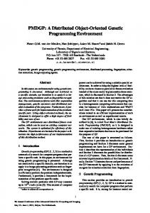
2.2 Overview of Neural Networks Neural networks (NNs) describes a method in connectionist machine learning. In NNs, the aim is to find values of parameters attached to a network of nodes that allow the correct output when a set of features is input.

2.2.1 Network Structure In many systems, a neural network is a network of nodes that is formed into a Directed Acyclic Graph (DAG), like that in figure 2.1. The nodes Output

w35 b3

4 b4

3 w23

w13 1

Output Layer

5 b5 w45

Hidden Layer

w14 w24 2

Input Layer

Figure 2.1: An example neural network.


16

of the network are arranged in layers. The bottom layer contains the input nodes, the middle layers contain the hidden nodes, and the top layer contains the output nodes. Each edge of the graph, called a link, carries a weight, which is a real value. Each hidden or output node in the graph carries a bias, which is a real value. There is one input node per feature in the task. The number of output nodes reflects the number of desired outputs.

2.2.2 Network Computations The aim of network training is to find a set of weight values that allows correct output when a feature-vector is input. Each node outputs a value to the nodes above it that are connected to it by links. Each input node outputs the value of a feature. The output of each node in the output and hidden layers in the network is computed from the values of the nodes in lower layers, according to equation 2.1 [17].

oi = f (

X

(wij vj ) + bi )

(2.1)

j

where the output of the hidden or output node i is oi . The bias of node i is bi . f is a transfer function such as a sigmoid. The sum covers all nodes j that input to node i. The weight between nodes i and j is wij . The output of the network is computed by computing the values of each node from the input nodes up.

2.2.3 Error Propagation Learning Method The common learning method for NNs is called the error propagation algorithm [37]. Error propagation uses the gradient-descent search method.

2.2. OVERVIEW OF NEURAL NETWORKS

17

Gradient-Descent When using gradient-descent, the gradient of a cost function is used to determine the relative changes to parameters in order to move to a lower cost. The lower cost means better performance at the task, and is often the Total Sum-Squared error (TSS) or Mean Squared Error (MSE). ∂C for all weights wij and a cost of C. The gradient vector includes the ∂w ij The values of the weights can be altered proportionally to the components

of the vector, leading to a lowering of the cost.

Error-Propagation The error propagation algorithm moves from the weights of the output ∂C layer down to the weights of the input layer. We can find ∂o for output oi i ∂oi ∂oi of any output node i. We can also find ∂oj and ∂wij for any node i receiving input from node j via weight wij , Using the chain rule, we can combine ∂C for any weight wij , which is what we require. these derivatives into ∂w ij

In [38], Rummelhart et al derived formulae for using error propagation in NNs. The change in a weight value wij is dependent on a learning rate η, an error value δj at the receiving node, and the output of the sending node oi . The formula is shown in equation 2.2. ∆wji = ηδj oi

(2.2)

The error δj is calculated using equation 2.3 for output nodes, and equation 2.4 for hidden nodes. δj = (tj − oj )fj′ (netj )

(2.3)

δk wkj

(2.4)

δj = fj′ (netj )

X k

where fj′ (netj ) is the derivative of the transfer function mapping the total input to a node to an output value. tj is the ideal value of an output node.


18

2.3 Overview of Evolutionary Computation While its origins were in the 1950’s [12, 13], Evolutionary Computation (EC) is recent as a recognized field. It is discussed here as a major contributer to the Genetic Programming (GP) method which is the topic of this thesis. This section seeks to review those areas of EC that are applicable to GP.

2.3.1 Evolutionary Computation Darwinian principles of natural selection form the primary inspiration for EC [49]. Although EC covers a wide range of methods, the common steps using EC are listed below: • Initial Population of Individuals The evolution starts with a collection, or population, of individuals. Each individual is a single point in the search space, and represents a potential solution to the problem. Often the initial population is comprised of randomly generated individuals. • Selection of fit individuals The fitness of individuals is evaluated at each time-step, or generation, during evolution. The fitness of an individual describes the individual’s quality as a solution to the problem. Fitter individuals are selected more often, and contribute more to later generations. • Generation of descendents In each generation, a new population is generated; it is comprised of a stochastically sampled set of individuals from the previous generation, biased towards those individuals of better fitness, after they

2.3. OVERVIEW OF EVOLUTIONARY COMPUTATION

19

have been altered using various operators such as mutation and recombination. Some good-fitness individuals may also be copied directly into the new population in order to prevent the best fitness from decreasing. Mutation is the random change of an individual to form a new individual that bears similarity to the parent. Recombination is the sharing of information from two individuals, producing new individuals that bear resemblance to both. The process of generating a new population from the previous is iterated for some number of generations. The process ends when an individual is found that is considered fit enough, a maximum number of generations occurs, or based on some other terminating criteria.

2.3.2 Aspects of EC In order to apply EC to a problem, various aspects of the method need to be addressed, which are discussed in the following sections.

Representation of Individuals Each individual contains a possible solution to the problem, and as such the representation used for individuals is vital to applying EC. Many representations have been used, from bit-strings and vectors of real values to more descriptive trees and graphs. The representation used must be descriptive enough to contain a solution to the problem, and concise enough to enable an efficient search. The representation used introduces a bias on the exact mechanism of the evolutionary search. For example, the search space of a fixed-length vector representation has a different shape to that of a tree representation, and this leads to a different bias in the evolutionary operators such as mutation.


20 Individual Fitness

The fitness, a measure of the quality, of any individual must be able to be computed. For example, an effective fitness mechanism for classification is the accuracy of the individual on the training set. Selection Mechanism The fitter individuals should contribute more than poorer individuals to later generations. This is achieved by the selection mechanism, which is used whenever selecting an individual for use in a new population. Many selection methods could be used, including proportional, rank, and tournament [28]. • Proportional Selection Proportional selection can be visualized as spinning a roulette wheel. The size of the segment on the wheel that applies to an individual is proportional to its fitness. As such, the probability of an individual being selected is proportional to its fitness. • Rank Selection When using rank selection, the rank of each individual is found, from first to last in the population. The probability of an individual being selected is based on a function of the rank of the invididual. • Tournament Selection When selecting an individual using tournament selection, the individual chosen is the one with the best fitness in a random group, of a set size, from the population. Producing a New Population Three methods can be used to produce a new population based on the individuals in the previous population: reproduction (direct copying of

2.3. OVERVIEW OF EVOLUTIONARY COMPUTATION

21

individuals), mutation and recombination. Evolution Control Parameters Some parameters must be set in order to use EC. These include the population size, termination criteria, and the proportion of the population coming from each operator. The parameters to evolution are often constant through evolution; however, some methods have changed parameters such as population size and mutation rate during evolution [25, 43].

2.3.3 Divisions in EC Four main methods derived from EC are: genetic algorithms, evolutionary strategies, evolutionary programming, and Genetic Programming (GP). The first three are described in this section, and GP is described in a separate section. Genetic Algorithms Genetic Algorithms (GAs) is an EC method developed in 1975 by J. Holland [18]. In GAs, the representation for solutions is typically a fixed length bitstrings, or chromosomes. While GAs use mutation and reproduction, a key distinguishing feature of GAs is the importance placed on crossover, which is used for recombination. Crossover involves exchanging regions of the parents’ chromosomes to form the children. Evolutionary Strategies and Evolutionary Programming Evolutionary Strategies (ES) and Evolutionary Programming (EP) were both created around 1964. Both use vectors of real values to represent individuals. In ES the individuals are used directly as solutions, in EP the


22

individuals are interpreted as finite-state machines. In both ES and EP, mutation is often the most important evolutionary operator.

2.4 Overview of Genetic Programming Genetic Programming (GP) is the method used in this thesis, and is a form of evolutionary computation. GP was first proposed by John Koza around 1989 [21, 22].

2.4.1 Program Representation The main differences between GP and GAs are the representation of individuals, called programs in GP, and the subsequent changes to the mutation and crossover operators. Several representations have been proposed for GP. Tree-Based GP The most common, and original, representation for GP programs is as trees, or LISP S-expressions; the tree-based representation and the LISP S-expression representation are interchangeable. A tree-based GP program is a single tree, an example of which is in figure 2.2. The internal nodes of the tree are functions. Each performs some function on the values coming from lower child nodes, and passes the result to its parent immediately above. The leaf nodes are terminals, which pass a value, such as a constant or feature value, to their parent node. The output of the root node is the program output. In the basic case, the values returned from nodes in a program are all of the same type, often floating-point numbers. In Strongly-Typed Genetic Programming (STGP) [5] this is not the case, and there exist functions that convert between types; an example is an if function that takes a boolean

2.4. OVERVIEW OF GENETIC PROGRAMMING

23

Output =3.2+(1.2*F1) +

3.2

Functions

*

LISP S−expression:(+ 3.2 (* 1.2 F1))

Terminals 1.2

F1

Figure 2.2: An example genetic program and its LISP S-expression.

and two floating-point numbers and returns either floating-point number depending on the state of the boolean. STGP allows for more natural use of some functions, such as conditionals, but adds complexity to the sets of functions and terminals used.

Linear GP Programs in Linear Genetic Programming (LGP) [4, 6] are variable length sequences of instructions from an imperative programming language. The instructions, or operations, perform some function on registers and constants, and assign the result to a register. For example, an operation could be r0 = r1 + 2. Conditional branches (such as if (r1 < r2 )) cause the next operation to be skipped. In LGP, programs may contain redundant operations, these are called non-effective, and can easily arise when, for example, a register is altered that does not affect the output. The operations that do affect the output are called effective. Separating the operations into effective and non-effective can be done in linear time and this algorithm is performed before program execution.


24 Grammar-based Representations

In Context-Free-Grammar Genetic Programming (CFG-GP) [55] program tree structures are evolved, similarly to in tree-based GP. However, the program trees evolved represent instances of a context-free-grammar (CFG). While the programs are not themselves evaluatable, they may easily be converted to the form of programs in tree-based GP for evaluation. The advantages of CFG-GP include: • Closure. In tree-based GP, the functions and terminals used must be chosen so that any combination of them can be evaluated. Due to the use of grammars, CFG-GP controls the shape of the program tree, and enforces that illegal combinations of functions and terminals do not occur. • Bias. Bias is easily introduced to the grammar used, allowing only those programs that are predicted to have better fitness. This is harder in tree-based GP. Grammatical Evolution (GE) [30] is a process inspired by the way a protein is generated from material in an organism’s DNA. A variablelength string of integers is parsed according to a Backus-Naur Form grammar (BNF), and forms an expression that may be evaluated. Definite Clause Translation Grammar Genetic Programming (DCTGGP) [35] evolves programs in the form of Definite Clause Translation Grammars (DCTGs). These grammars include not only the context-free information of CFGs, but also context-sensitive information as to the semantics of the grammar. This allows more difficult legality checks to be placed on a program than those of other systems, however these checks require additional system components to enforce. The tree-based method is the approach used in this thesis. In the following sections we describe the aspects of tree-based GP.


25

2.4.2 Program Generation The initial population of individuals in GP is commonly made up of randomly generated individuals. For the basic approach, all functions and terminals return the same type, and so any function can take any function or terminal as its children. Generating a Single Program Two methods may be used to generate a random tree or subtree: full or grow [22]. • Full Method Using the full program generation method, functions are randomly selected to be the nodes of the tree, starting at the root and moving down the tree by filling up layers. At a set depth, the tree is finished by fitting terminals to all inputs of the lowest level functions. • Grow Method Using the grow program generation method, the nodes of the tree are randomly selected as functions or terminals, starting at the root and moving down the tree by filling up layers. This continues until there are no leaf functions, or to a set depth; if the depth is reached, the tree is finished by fitting terminals to all inputs of the leaf functions. Generating a Population of Programs The initial population in GP is often made up of randomly generated programs. Although either of the full or grow program generation methods could be used for all programs in the population, the population is more often comprised of a combination of full and grow programs. • Half-and-half


26

In the half-and-half method, half the population is formed from full and half from grow. • Ramped Using the ramped method, the maximum tree depth is increased from some minimum value to a maximum value; each value has an equal proportion of generated programs. A common method is the combination of all these techniques in ramped half-and-half [22].

2.4.3 Genetic Operators The genetic operators of GP are the same as in GAs: reproduction, mutation and crossover. Reproduction To ensure that the fitness of programs in a population is never less than that of previous generations, the reproduction, or elitism, operator is used. This consists of simply copying the best few programs of a generation’s population directly to the next. Mutation In mutation, a single program is selected from the population and copied to a mating pool. A mutation point is chosen randomly, somewhere in the program, and the subtree below the mutation point is replaced with a new, randomly generated subtree. The new program is then copied into the new population. This is pictured in figure 2.3. Mutation is used to ensure diversity of programs in the population and for introducing new genetic material.


27

Mutation point +

+

3.2

3.2

*

F1

1.2

+

F3

F2 Random

Parent

Child

Figure 2.3: Mutation genetic operator. Crossover In crossover (or recombination), two programs are selected from the population, both are then copied to a mating pool. A crossover point is randomly chosen in each program, and the subtrees below the crossover points are swapped. The two programs, with swapped subtrees, are then copied to the new population. This is pictured in figure 2.4. Crossover points +

3.2

+

3.2

*

1.2

F1

Parents

+

F2

3.2

+

3.2

*

1.2

F2

F1

Children

Figure 2.4: Crossover genetic operator.

Crossover is used to allow mixing of material from two programs into one program.


28

2.4.4 Current Issues in Genetic Programming

Although a recent technique, GP has proven to be remarkably flexible in application. However, as with other machine learning methods, GP has some limitations. The search space of programs used by GP is often huge, and learning can often be slower than other methods. As such, work is being done on Parallel Genetic Programming (PGP) [11, 52], where evolution progresses on multiple processors simultaneously. PGP has emerged in two main varieties: island, where semi-separate populations called deems are used, and grid or cellular, where the individuals in the population are arranged spatially in a grid. The representation of individuals in GP has received much attention in recent research, as the standard representations are not applicable to all problems. Some new representations include: linear programs [4, 6], Finite State Transducers (FSTs) [26], and cellular automata [40]. One problem that may occur in a GP system is bloat, or code growth, where the size of programs tends to increase as evolution progresses. Bloat can make the search harder for the GP system, as the larger programs increase the size of the search space, and size limits may be reached, impeding further search. Much recent research has been performed to determine the cause of bloat [7, 47, 48] and reduce it [32, 27]. The use of other search techniques, in addition to the evolutionary search in GP, has been the subject of recent research. Such approaches include: the use of a global GP search with a local gradient-descent search of constants or numeric terminals [42, 53], the use of a global meta-search with a local GP search [23], and using an evolutionary search to evolve Neural Networks (NNs) [8, 57, 58].

2.5. OVERVIEW OF OBJECT CLASSIFICATION

29

2.5 Overview of Object Classification 2.5.1 Object Classification Object classification is the problem domain of this thesis, and is a supervised machine learning problem. The training data for the classifier includes vectors of features, with each having a target class label. The test data are feature-vectors from the same source. The class labels of the test set are known, but are not used for training; the test data is unseen data, which is used to evaluate the performance of the system. The aim of the classifier is to be able to correctly identify the class labels of the test data, based on knowledge learned from the training data.

2.5.2 Aspects of Object Classification Object classification has a number of important aspects in its application, such as the number of classes, level of features, and performance evaluation. Number of Classes Binary classification problems are those that distinguish only two classes. In contrast, multiclass classifiers must distinguish between more than two classes. The number of classes that a classifier is expected to distinguish is partly problem-dependent. However, problems with large numbers of classes may safely be broken into multiple problems that distinguish between subsets of the total set of classes [2]. Level of Features The feature-vectors in object classification are computed from objects in images. As the object is an image, many different types of feature can be


30

used, from direct pixel values through to very domain-specific high-level features. • Pixel-level features The lowest level feature is the pixel value, used directly as a features [46]. Due to the fact that all images are made up of pixels, this is the most domain-independent form of feature. When using pixel features, the feature-vector will typically be very large, as even the smallest image typically has in excess of 100 pixels. • High-level features Some approaches use very high-level features [50]. There are many high-level features that are able to be derived from an image, and some are very descriptive of the contents of the image. However, these features may be domain-dependent, and certain domain knowledge is required in their use. For example, some high-level features that can be used in texture classification are the Grey Level Co-occurrence Matrix (GLCM) features. • Pixel-statistic features Recently, statistics from regions of pixels in the object images have been used as the features [24, 62, 59]. These statistics, such as variance and mean, aim to reduce the number of required features, while still being domain-independent. Pixel-statistics may also be made invariant under rotation or translation. Performance Evaluation Typically, the method for evaluating the quality of a classifier is to compute its accuracy on a large number of objects. The accuracy of a classifier is the proportion of object classes that it predicts correctly in a set of data. As such, 100% is the perfect accuracy, and 0% the worst.

2.6. RELATED WORK TO GP FOR IMAGE RECOGNITION TASKS

31

Other measures of the performance of the classifier include Total SumSquared error (TSS) and Mean Squared Error (MSE).

2.5.3 Current Issues in Object Classification Some current issues to do with classification include: • There are a number of emerging applications. Due to the increasing ability of computers, classification tasks are emerging from many areas such as bioinformatics, computer vision, the Internet, and economic forecasts. A large number of new data sets have been made available for processing. Much of this data requires classifiers, for example whether to buy or sell stocks in a company, given its financial figures. • The representation of classifiers is important. There are many structures that can classify, such as decision trees, neural networks and genetic programs; which is best is the subject of much research.

2.6 Related Work to GP for Image Recognition Tasks This section presents a review of the most relevant literature where GP was applied to image object recognition tasks. The tasks of GP where images are concerned mainly include classification, detection, localization, and image processing. Localization is the process of finding an object in an image; detection can be thought of as combining localization and classification.


32

2.6.1 Localization and Detection In [51], Tackett located targets in images using binary tree classifiers, NNs, and GP. The GP method was found best for performance and computational efficiency. A large data set was used, and pixel level features outperformed pixel-statistics, possibly due to the segmentation artifacts, and lower resolution, of the pixel-statistics. In [61], Zhang and Ciesielski used GP and NNs to detect objects in a range of data sets. A small window was passed over all areas of the images, with program fitness using both detection rate and false alarm rate. While GP results are better than those of NNs, many errors are still found with the method on the more difficult problems. In [20], Johnson used GP to evolve hand detectors for silhouette images. Results were promising, with the GP evolved detectors outperforming hand-coded detectors. In [56], Winkeler et al. used GP to detect faces. The GP system was trained on pixel-statistics obtained from face and non-face regions in the images. Results were mixed, and an issue was found in trying to indicate training set non-objects.

Remote Sensing In [9], Daida et al. used a method including GP to extract ridge and rubble locations in Synthetic Aperture Radar (SAR) images of multi-year sea ice. Excellent results were produced, good enough to detect gross deformation patterns between images taken at different times. In [19], Howard et al. used methods, including GP, to detect ships in SAR images. GP compared favourably against rival methods; the low complexity, and high efficiency, of the detectors evolved was seen as an advantage over methods such as NNs.

2.6. RELATED WORK TO GP FOR IMAGE RECOGNITION TASKS

33

2.6.2 Classification In [36], Ross et al. used GP with high-level features to produce classifiers, which identified minerals in hyperstectral images. Each classifier determined existence of a particular mineral. The approach gained good performance, especially for minerals with high reflectance. The requirement for a good training set was noted. Song classified textures using pixel features in [45]. Two approaches were used: one approach extracted texture features, and another used pixel-level features. On the simple tasks attempted, the GP method faired well against another method (C4.5). In [1], Agnelli et al. used GP to classify images of documents into the categories of picture, or text. The results were good. The resultant programs were thoroughly examined, and found to carry fairly simple rules in solving the task. In [3], Andre used GP to generate rules to identify images of the letter ‘C’. The programs produced could perfectly classify examples in the trained font, but did not generalize to other fonts as well as hand coded classifiers. The understandability of the produced rules, and their ability to be translated into the programming language C, were key points in the design.

2.6.3 Image Processing In [15], Harris et al. evolved edge detectors for 1D signals using GP. Several detectors were found that outperformed Canny’s approximation to the optimal detector. In [31], Poli gained impressive results using GP to segment Magnetic Resonance (MR) medical images. GP was compared to NNs, and produced much neater segmentation, although the computationally expensive training was an issue. In [34], Roberts et al. used GP to evolve programs that can determine


34

the orientation of an object in linescan imagery. The novel method produced very robust detectors.

2.7 Related Work to GP for multiclass Object Classification A small amount of work has been done in GP on classifying objects into more than two classes. In [24], Loveard applies GP to several binary and multiclass medical data sets. Various classification strategies are used for converting the output of a program into a class value. The methods of binary decomposition, static range selection, dynamic range selection, class enumeration and evidence accumulation are described. Dynamic range selection was found to be the method with the best mix of speed and accuracy. In [41], Smart et al. use GP on multiclass object classification problems. Two classification strategies, centred dynamic range selection and slotted dynamic range selection, are introduced. The new strategies outperformed the more basic static range selection on more difficult problems with many classes. In [44], Smith et al. use GP and C4.5 to classify patterns in several binary and multiclass medical data sets. GP was used to evolve high-level features, which were then passed to a C4.5 classifier. The method was found to significantly improve the accuracy of the C4.5 classifier, compared to its use alone.

2.8 Summary and Discussion This chapter presents a review of the fields that are relevant to the work in this thesis, including: machine learning, evolutionary computing, neural networks, genetic programming and classification. The related work of

2.8. SUMMARY AND DISCUSSION

35

genetic programming for image recognition tasks is also discussed. A summary of the current state in these areas is as follows: • GP has emerged as a rapidly growing method that has performed favorably against rival methods in a number of tasks: these include classification, and image related tasks of detection, classification, and image processing. • Very little work has been done to apply GP to multiclass object classification problems, and the problem of converting program results to class labels (that of classification strategies) is unsolved. • A potentially large research area of hybrid search methods, combining the GP evolutionary search with other search schemes, has had little attention. This thesis addresses the areas of classification strategies, and use of gradient-descent search in GP.

36


Chapter 3 Data Sets The methods within this thesis are applied to multiclass object classification tasks. This chapter describes the data sets comprised of the objects to be classified. Three sets of images with objects were used. For each set of images a number of compound images, each with many objects, were acquired either through rendering or scanning. The objects in the images were manually located and cut out, forming a great number of small cutout images, each with a single, centred object. The classification task is to determine the class of these objects, when given only the cutout images. The three sets of images were formed into four multiclass tasks, or data sets.

3.1 Image Content Three sets of images were used: • Shapes: Computer generated shapes drawn with a Gaussian filter. • Coins: New Zealand ten and five cent coins. • Faces: Faces of four people. 37

CHAPTER 3. DATA SETS

38

3.1.1 Shapes Example ‘Shapes’ images are shown in figure 3.1, along with an example of each of the three classes.

1/24

2/24

Class 1

Class 2

Class 3

Figure 3.1: Shape images and classes. The images for the ‘Shapes’ images are computer generated. Each image contains ten each of black circles, dark-grey squares, and light-grey circles. The objects are drawn using a Gaussian filter against a speckled white background. The object of each class in this data set are well separated into different intensity ranges. As such, the classification task of distinguishing between the classes is expected to be easy.

3.1.2 Coins Example ‘Coins’ images are shown in figure 3.2, along with an example of each of the five classes. The ‘Coins’ images are comprised of scanned images of New Zealand

3.1. IMAGE CONTENT

39

10c coins

Class 1

10c and 5c coins

Class 2

Class 3

Class 4

Class 5

Figure 3.2: Coin images and classes.

coins. The five classes in the Coins images are: the background, five-cent tails, five-cent heads, ten-cent tails, and ten-cent heads. The coins featured in this set of images are less well defined than the objects of the ‘Shapes’ images. The coins are featured against a background of similar intensity to the coins themselves, and the differences between the classes of coins are less visible than the clear distinction between the classes of the ‘Shapes’ images. As such, the coins classification task is expected to be harder than that of the ‘Shapes’ images. The coins are still clearly man-made objects. The only changes made to images of a class of coin, from one object to the next, were the orientation and background. So the coin images of each class would look the same if segmented and rotated upright.


40

3.1.3 Faces The final set of images were obtained from the ORL face database [39] from which only the first four classes were used. The entire set of images is shown in figure 3.3.

Figure 3.3: Face data set images.

The four classes relate to four people, each of whom has ten cutouts. The classification problem is made harder by varying orientation, expressions (smiling, open-mouth, etc.), and accessories (glasses on, glasses off) of the people between images. Also, some images feature minor changes to lighting. This task features complex objects with little difference between the objects of different classes, and some wide variability within objects of the same class. The faces do not have the same similarity between objects of the same class as the previous sets of images. As such, this is expected to be a more difficult classification task than that of the previous two sets of images.

3.2. DATA SETS

41

3.2 Data Sets The three sets of images were made into four data sets for experiments: • Four-class Shapes: All four classes of the Shapes images. Because the intensities of the objects are well separated into classes, we expect that this is a relatively easy classification task. • Three-class Coins: The first three classes of the Coins images. This classification task uses the Coins set of images, which is expected to be more difficult to classify than the set of Shape images. • Five-class Coins: All five classes of the Coins images. This classification task is expected to be harder than the previous two, both because of the noisy and difficult to discern source of the objects, and because of the larger number of classes. • Four-class Faces: All four classes of the Faces images. Of the four data sets used, the Faces data set is expected to be the hardest due to the complexity of the objects. Table 3.1 lists the number and size of cutouts in each of the data sets. Table 3.1: Number and size of data set cutouts. Data set

Classes

Cutouts of each class

Size of cutouts

Shapes

3

240/240/240

16×16

Three-Class Coins

3

192/192/192

70×70

Five-Class Coins

5

96/96/96/96/96

70×70

Faces

4

10/10/10/10

90×110


42

3.3 Training, Test and Validation Sets The objects of each data set were split equally into three sets (except for the Faces data set): • Training set: the evolutionary process may use the class labels of this set in order to train, learning the relationship between class labels and features. • Test set: the evolutionary process may use the class labels in this set only once per evolution, and only in order to find classifier accuracy.

• Validation set: the evolutionary process may use the class labels of this set; however it is kept at arms length. This set is used to find the generation at which to calculate the test set accuracy, which should be done only once. The validation set accuracy is calculated once per generation. At the end of the run the generation of best such accuracy is the generation in which the test set accuracy is measured. This mechanism controls overfitting, where the accuracy of the current best classifier on unseen patterns may fall in later generations. If over-fitting occurs, the final test accuracy would be worse than some previous generation’s test accuracy, but the same would be true of the validation set accuracy. Taking the test set accuracy at generation of best validation set accuracy is a means to report the best possible test set accuracy for the run, while only (if retrospectively) taking the test set accuracy once. Due to the small number of objects of each class in the Faces data set, ten-fold cross-validation was used in all Faces data set experiments. This precluded the use of a validation set as used elsewhere. The test set was substituted for the validation set in experiments using the Faces data set. This means that, where a result is quoted at the generation of best validation set accuracy and the result uses the Faces data set, the result is in fact as at the generation of best test set accuracy.

Chapter 4 Basic Approach This chapter will describe the basic methodology used when the standard GP approach is applied to multiclass object classification problems.

4.1 Introduction In this thesis, new methods using GP for multiclass object classification problems are described. Often the goal of a new method is to improve the performance of the classification system, against a basic approach. This chapter describes this basic approach, which is a system that uses GP in a standard way to solve the multiclass classification problem. In later chapters, the performances of new methods will be compared to the baseline performances in this chapter; in so doing, we hope to evaluate how much the new methods improve performance over the standard approach.

4.1.1 Goals This chapter aims to achieve the following goals: 1. To define a standard approach to GP for multiclass object classification. 43

CHAPTER 4. BASIC APPROACH

44

2. To serve as a baseline for comparison to new methods, enabling measurement of the improvement in performance of a new method over standard GP.

4.2 Primitive Sets 4.2.1 Features Used In this approach, four simple pixel statistic features were extracted from the object cutouts. These formed the feature vectors used as input to the programs. The pixel statistic features come from two regions in the cutouts (whole cutout and centre quarter) and are of two types (mean intensity and standarddeviation of intensity). Figure 4.1 shows the regions used and table 4.1 lists the combinations used as the four features.

A

h/4

E

F h/2

w/4

H D

B

h

G w/2

C

w

Figure 4.1: Regions used for cutouts.

4.2.2 Terminal Set The terminals used in the evolved programs include numeric terminals and feature terminals.

4.2. PRIMITIVE SETS

45 Table 4.1: List of features.

Feature number

Region in figure 4.1 Pixel statistic type

1

Area inside ABCD

Mean intensity

2

Area inside ABCD

Std. dev. of intensity

3

Area inside EFGH

Mean intensity

4

Area inside EFGH

Std. dev. of intensity

Feature Terminals Each feature terminal returns one of the features described previously. For a particular feature terminal node, the number of the feature returned is selected randomly, and does not change during evolution. Numeric Terminals Each numeric terminal returns a randomly assigned constant value. The value is sampled from a standard normal distribution (mean of zero, standard deviation of one). For a particular numeric terminal node, the value returned does not change during evolution.

4.2.3 Function Set In the basic approach, simple arithmetic operators were used as functions, along with conditional operators. The functions are displayed in table 4.2. In the table, ai indicates the value of the i’th argument to the function. The exact functions used depend on the method that is being compared to the new method. To enable a fair comparison with a new method, when comparing it to the basic approach, both approaches use the same function set.


46

Table 4.2: Function set. Function

Symbol

Addition

+

2 a1 + a2

Subtraction

−

2 a1 − a2

×

2 a1 a2

Negation Multiplication Protected

Num. args.

neg %

1 −a1

2

a1 a2

if a2 6= 0

0 if a2 = 0

Division Protected

Formula

inv

1 a−1 1 if a2 6= 0 0 if a1 = 0

Inversion

a2 1+e2a1

+

a3 1+e−2a1

Soft Conditional

sif

3

Conditional

if

3 a2 if a1 < 0 a3 if a1 ≥ 0

4.3 Fitness Function In the basic approach, PCM is used as the classification strategy, and accuracy as the fitness function.

4.3.1 Program Classification Map A simple and widely used classification strategy is Program Classification Map (PCM), developed in [60]. A variation of PCM has been called Static Range Selection (SRS). The space of the floating-point program output is divided into a set of regions. The whole space is covered, and no part of the space is covered twice. There are exactly the same number of regions as classes in the classification problem, with each region mapped to a different class. The regions are situated between a series of thresholds, t1 ..tN −1 where

4.3. FITNESS FUNCTION

47

N is the number of classes. The rule that ti < ti+1 is enforced for all 1 ≤ i < N − 1. The first region includes the space [−∞,t1 ) for class one. The final region includes the space [tN −1 ,∞] for class N. All other regions occupy the space [ti−1 ,ti ) for class i. Any point on the real number line is unambiguously associated with a region, and with it a class label. A program that produces an output, when given a feature-vector as input, can therefore associate the output with a single class label. Thus, the feature-vector is classified as the class label associated with the output. An example map with four classes is shown in figure 4.2.

Class 1

2

−1

4

3

0

1

Figure 4.2: An example program classification map for four classes.

In the figure the thresholds between the regions are laid out on the real number line at a spacing of one unit, between a negative number and the same number as a positive. This is the class layout used in basic approach experiments.

4.3.2 Accuracy Fitness Function The fitness function used is training set accuracy, which is the fraction of training set objects correctly classified by an evolved program. As such, zero is the worst possible fitness, and one the best possible fitness for a program.


48

4.4 Parameters and Termination Criteria Table 4.3 lists the parameters used inside the GP engine for all experiments. Table 4.3: Common GP Parameters for Experiments. Parameter Kinds Parameter Names Values Search

Parameters Genetic Parameters

population-size

250 or 500

initial-max-depth max-depth max-generations

4 7 50 or 100

reproduction-rate crossover-rate mutation-rate

10% 60% 30%

crossover-term crossover-func

15% 85%

Programs were created using ramped-half-and-half program generation.

4.4.1 Termination Criteria All basic approach experiments were run with early-stopping; the training was stopped once an individual was produced with the ideal fitness (1.0). In case this had not happened before the maximum number of generations, training was stopped at that point.

4.4.2 Performance Evaluation All experiments were run fifty times, with no change in parameters except the random seed used. The results shown are the mean (and standard

4.4. PARAMETERS AND TERMINATION CRITERIA

49

deviation) over the fifty runs. The random seed contributes to all random processes in evolution, such as program generation and selection. Using the mean over fifty runs is an attempt to remove the effect of these random processes from the results, so that the results focus only on the specific performance of the method used for evolution. Results Displayed The results that are displayed include the following: • Total Evaluations: The number of evaluations of nodes performed in the whole run of evolution. • Final Generation: The number of generations in the whole run of evolution. • Run Time: The total time per evolutionary run. • Final Test Accuracy: The accuracy of the run’s final generation classifier.

• Evaluations at Best Validation Accuracy: The number of evaluations of nodes performed in the run up until the generation that had the best validation set accuracy.

• Generations at Best Validation Accuracy: The run’s generation of best validation set accuracy. • Time at Best Validation Accuracy: The time taken in the run to obtain the best validation set accuracy. • Test Accuracy at Best Validation Accuracy: The test accuracy at the generation of best validation set accuracy.

For presentation convenience, a result that is “at the best validation set accuracy” will be referred to as “at convergence”.


50

4.5 Experimental Variations In this thesis, the basic approach is compared to the new approaches. The different chapters have slight changes to the experimental setup due to the requirements of the method being compared. In total, there are three such variations in experimental setup: • Chapters 5 and 6 use a population size of 500, a maximum of 50 generations and a function set containing {+, -, *, %, sif }. • Chapter 7 uses a population size of 500, a maximum of 50 generations and a function set containing {+, -, *, %, if }. • Chapter 8 uses a population size of 250, a maximum of 100 generations and a function set containing {+, *, neg, inv}.

4.6 Results and Analysis This section displays the results obtained in the basic approach experiments. Tables 4.4 and 4.5 display the results of the basic approach for each data set and experimental setup. Table 4.4 displays the results for the final generation of each run. From table 4.4 it is seen that the basic approach could not solve the ‘Five-Class Coin’ problem within the maximum number of generations, and seldom solved the ‘Faces’ problem. Table 4.5 displays the results for the generation of best validation set accuracy. As expected, it is seen from table 4.5 that the ‘Faces’ and ‘FiveClass Coin’ data sets achieved worse accuracy than the two other data sets. However, the ‘Shapes’ data set is seen to have lower accuracy than the ‘Three-Class Coins’ data set in both tables of results. Also, the ‘Faces’ data set is seen to have better accuracy than the ‘Five-Class Coins’ data set at convergence. This is probably due to PCM, which suffers as more

4.6. RESULTS AND ANALYSIS

51

Table 4.4: Basic approach results at final generation.

Dataset

Function

Max.

Pop.

Total evals.

Final

Run

Final test acc.

Set

Gens.

Size

(x1M)

gen.

time (s)

(%)

Shapes

+,-,*,%,sif

50

500

127.54

13.32

2.62

4 class

+,-,*,%,if

50

500

230.84

23.76

1.94

99.68 ± 0.51

+,*,neg,inv

100

250

96.57

50.94

1.00

Coins

+,-,*,%,sif

50

500

58.80

11.16

1.33

3 class

+,-,*,%,if

50

500

82.12

16.90

0.86

+,*,neg,inv

100

250

53.47

53.68

0.65

Coins

+,-,*,%,sif

50

500

265.41

50.00

6.17

5 class

+,-,*,%,if

50

500

274.19

50.00

3.07

+,*,neg,inv

100

250

97.65

100.00

1.25

Faces

+,-,*,%,sif

50

500

56.23

49.92

2.26

4 class

+,-,*,%,if

50

500

58.07

49.84

1.73

+,*,neg,inv

100

250

20.54

100.00

0.64

99.62 ± 0.76

97.86 ± 3.87

99.59 ± 0.60 99.65 ± 1.33

98.85 ± 1.06

74.44 ± 8.07 85.54 ± 6.35

66.07 ± 5.29

71.60 ± 17.84 73.50 ± 18.24

71.65 ± 15.41

classes are introduced to the problem as the programs must deal with a specific order and placement of the class regions. The ‘Faces’ data set is seen to converge much earlier than the ‘FiveClass Coins’ data set. It is seen from the tables that the choice of negation and inversion in the function set, in place of subtraction, division, and a conditional, impeded performance in terms of accuracy and efficiency. This may be due to the depth limit enforced on programs, as well as the usefulness of the conditional function. A tree of the same depth may be more expressive when using subtraction and division, than when negation and inversion are used. Using sif in the function set is seen to give similar accuracy to the use of if , but usually causes longer run times. However, for the ‘Five-Class Coin’


52

Table 4.5: Basic approach results at generation of best validation set accuracy.

Dataset

Function

Max.

Pop.

Evals. at best

Gens at

Time at

Test acc. at

Set

Gens.

Size

val. (x1M)

best val

best val.

best val (%)

Shapes

+,-,*,%,sif

50

500

116.26

12.22

2.39

4 class

+,-,*,%,if

50

500

201.68

20.96

1.70

99.67 ± 0.55

+,*,neg,inv

100

250

64.85

36.60

0.68

Coins

+,-,*,%,sif

50

500

42.98

8.74

0.95

4 class

+,-,*,%,if

50

500

64.24

13.74

0.67

+,*,neg,inv

100

250

20.65

24.60

0.27

Coins

+,-,*,%,sif

50

500

190.90

37.18

4.43

4 class

+,-,*,%,if

50

500

231.36

42.80

2.60

+,*,neg,inv

100

250

49.79

53.28

0.64

Faces

+,-,*,%,sif

50

500

6.82

6.75

0.26

4 class

+,-,*,%,if

50

500

11.22

10.57

0.32

+,*,neg,inv

100

250

1.36

8.38

0.04

99.56 ± 0.83

97.82 ± 3.90

99.44 ± 0.88

99.56 ± 1.36

98.79 ± 1.25

74.40 ± 7.98 85.29 ± 6.40

65.26 ± 5.62

82.15 ± 13.61 81.40 ± 14.46

79.70 ± 13.05

data set, the use of sif gave much worse accuracy than the use of if . This may be due to the need for sharp cutoffs between the five classes, which are arranged into definite regions on the real number line. sif cannot give a sharp discontinuous cutoff between classes, and so may have lowered accuracy when there were many classes.

4.7 Chapter Summary The goal of this chapter was to define a standard approach to GP for multiclass object classification which would serve as a baseline for comparison to new methods, enabling measurement of the improvement in performance of a new method over standard GP.

4.7. CHAPTER SUMMARY

53

The method of this chapter may be described as a standard way to use GP for multiclass object classification. In later chapters this method will be compared to the new methods, indicating any increase or decrease in performance compared to standard GP.

54


Chapter 5 Probabilistic Classification Methods In this chapter we propose a new method for interpreting a GP program result as one of a set of classes.

5.1 Introduction and Motivation Classification is a basic problem in artificial intelligence, and often takes the form of predicting the class of a vector of feature values. In order to perform classification using GP, a program is sought that can take the feature values as inputs and produce an output that relates to the class. While the features can easily be input into such a program, difficulties arise when interpreting the output of a program as a class: in most treebased GP implementations a program can only output a single floatingpoint number. The problem of determining the class of a floating-point number is the subject of this chapter. Here, a solution is termed a classification strategy. Many classification strategies have been created in the past allowing GP to be used for multiclass classification. However, most previous methods had disadvantages when compared to the new, probabilistic, method de55

56

CHAPTER 5. PROBABILISTIC CLASSIFICATION METHODS

scribed in this chapter. These disadvantages may include: • Parameters to set Some classification strategies have many parameters to set in their use. Setting many parameters may involve a lengthy empirical search for their values. • Constraints on the evolved programs Some classification strategies place constraints on the evolved programs, over and above those necessary to classify the objects. Placing heavy constraints on the evolving programs may result in a small number of programs that can both solve the classification problem, and satisfy the constraints. This may cause low performance. • Little mathematical basis Mathematics can guide the process of making a new method, and is often a desirable attribute of a method. The new method, Probabilistic Multiclass (PM), described in this chapter aims to avoid the disadvantages of other classification strategies. It differs from previous approaches by its probabilistic model for the program output distribution. This model is seen to place fewer constraints on programs than previous methods while still allowing programs to be effective in solving the classification task. The result is faster convergence and higher test set accuracy. Another advantage of the method is that multiple best programs, each with different strengths, can be mathematically combined to form a stronger classifier, that may outperform any one of the best programs by itself. The remainder of this chapter starts with the chapter goals, followed by the background of the classification strategy problem, with some previous methods described. Section 5.4 describes the new probabilistic model for program output, and section 5.5 describes the new classification method using this model, Probabilistic Multiclass (PM). In section 5.6 the results

5.2. CHAPTER GOALS

57

of some experiments evaluating the new method are displayed and analyzed. Section 5.7 summarizes the chapter and discusses the effectiveness of the new method.

5.2 Chapter Goals This chapter aims to address the first hypothesis given in section 1.1.1: Will a new GP method with a probabilistic classification strategy outperform the basic GP method on a sequence of multiclass object classification problems? This research question is broken up in this chapter to the following finer research questions: • How can a probabilistic model be developed for the output distribu-

tion of a program on training data, allowing the classes to be distinguished?

• How can the fitness function be constructed using the probabilistic model? • How can the classification accuracy be calculated using the probabilistic model?

• Will the method achieve better performance than the basic approach on a sequence of multiclass object classification problems?

5.3 Background The output of a genetic program is usually a single floating-point number; classification requires a discrete class label to be assigned. A function f : R → S is required, where R is the set of real numbers, and S is a set of class labels with one member per class in the classification problem. The function will take the output of a program, and convert it to a class label.

58


Several classification strategies have been developed to solve this problem, and the remainder of this section describes some of these.

5.3.1 Program Classification Map A simple and widely used classification strategy is Program Classification Map (PCM), developed by Zhang [60]. It was described in detail in section 4.3.1. The space of the floating-point program output is divided into a set of regions. There are exactly the same number of regions as classes in the classification problem, with each region mapped to a different class. While PCM is easy to implement and explain, it often tends to have low performance. PCM forces all programs to output into the same regions, so all programs are constrained to have the same output distributions. The regions are set by the user, and while possibly not obvious to the user, may be important to the performance of evolution. The order of the classes in the data set may also be important to performance.

5.3.2 Centred Dynamic Range Selection Centred Dynamic Range Selection (CDRS) is based on PCM, but requires less domain-specific knowledge to operate. CDRS was developed in the author’s honours project. CDRS uses a dynamic classification map. The type of map is the same as that of PCM, however the order and position of the classes will normally change from generation to generation. The average return value for each class, using all programs on all training data, is found periodically during evolution. The thresholds, as used in PCM, are set halfway between adjacent class averages. An advantage of CDRS is that it requires few parameters to be set by the user. Also, the order and position of class regions is automatically defined by the algorithm.

5.3. BACKGROUND

59

A disadvantage of CDRS is that it still forces all programs to share a single classification map. The map is found by an average, so even if 95% of programs are very bad at the task, these 95% will still dominate the calculation for the classification map. Another disadvantage is the complexity of the calculation for the class thresholds, which can sometimes cause undesired behaviour such as oscillations and excessive shrinking of some class regions.

5.3.3 Slotted Dynamic Range Selection Slotted Dynamic Range Selection (SDRS) from [41] was based on Dynamic Range Selection (DRS) in [24]. In SDRS a number of non-overlapping, same-sized regions (called slots) are assigned to cover a portion of the real number line. There are a large number of slots and they are intended to cover a large area of the real number line, where most program results fall. Each of the slots is assigned a class value. A program result that falls into a slot classifies as the class assigned to the slot. An example slot map is shown in figure 5.1

Class 1

Class 3

Class 2

Class 4

−100

0

100

Figure 5.1: An example slot map for SDRS. The class of each slot is reassigned periodically during evolution. For each class, all programs are evaluated on all training examples of the class. This produces a set of program results for each class. For each slot, the members of the sets of program results are checked to see if they fall into the slot. The class of the set that has the most program

60


results that fall into the slot is assigned as the slot’s class. For example, if the training examples of class two often fall into a particular slot, and not many examples of the other classes fall into the slot, then the slot will be assigned class two. Some advantages of SDRS are the very complex class maps possible, and that it requires very little domain knowledge from the user as the class mapping is found automatically. Some disadvantages of SDRS are that it still forces all programs to share a common map, and the complexity of the map can cause irregularities when used with small datasets. DRS does not force all programs to share a common classification map, but still suffers from irregularities in the map due to small data sets. Also, there are several parameters such as the quantity and placement of the slots that need to be set with SDRS. Finding good values for these may require a lengthy empirical search.

5.4 Probabilistic Model of Program Output While the aim of a classification strategy is to produce a function f : R →

S for each program, the new method does not deal with this function directly (as do PCM, CDRS and SDRS). Instead, the function is derived from a higher level model of the program’s output.

5.4.1 Foundation for the Model Some assumptions are made about the output distribution of a program that is good at the classification task. These allow us to model the distribution. 1. The first assumption is that a good program will produce similar outputs when evaluated on examples of the same class. 2. The second assumption is that a good program will produce distant outputs for examples of different classes.

5.4. PROBABILISTIC MODEL OF PROGRAM OUTPUT

61

3. The third assumption is that the distribution of outputs of a program, for a large enough set containing examples of only one class, may be reasonably modeled by a single normal curve. Based on these assumptions, a program output distribution can be modeled as a mixture of normal distributions, with one per class in the classification problem. Figure 5.2 shows an example, with a program output modeled for a dataset of three classes. Class 3 Class 1

Class 2

10.0 −10.0 −5.0 0.0 5.0 Figure 5.2: Probabilistic program output model example.

In figure 5.2 the output distribution of a program has been modeled by three normal curves. From the model, class one tends to produce lower output than the other two classes, with class three next, then class two. Also, the output of the program for class one is less centralized than the other classes, with a lower, wider curve. It is easy to see how such a model simplifies dealing with the program’s output distribution on a large data set. Advantages of the Model The advantages of this model for a program’s output distribution are described as follows: • Normal distributions are possibly the most common distribution found in natural data, and so could be expected to fit program output well. • Normal distributions are easily found from data, and have a good mathematical foundation for calculations.

62

CHAPTER 5. PROBABILISTIC CLASSIFICATION METHODS • Modeling a program’s output distribution as just a few normal distributions restricts the complexity of the model. This may help reduce over-fitting and the irregularities of class regions along the real number line found with some classification strategies, such as SDRS. • Multiple programs can be combined together when using the probabilistic approach. This gives the opportunity for different programs to combine their strengths, as an form of ensemble method.

Restrictions of the Model The assumptions restrict the programs in two ways: the number of clusters of program outputs for a class, and the shape of the clusters. They are shown graphically in figure 5.3. Both class 1 Mean

1.2 Class 2

6.3 (a)

11.4

(b)

Figure 5.3: Badly fitted program output distributions. The model allows only one cluster of program outputs per class for a program, as the output is modeled by a single normal curve. As such, the model does not allow a program to, for instance, output values around 1.2 for half of the examples of a class, and around 11.4 for the other half. In such a case (shown in figure 5.3(a)), the normal model of the program’s

5.4. PROBABILISTIC MODEL OF PROGRAM OUTPUT

63

output for the class would have a mean around 6.3 and would fit the actual output distribution quite badly. The second restriction is the shape of the distribution of program output for each class, which is assumed to be a normal distribution. Though one can think of examples where such a distribution could be off normal for some program (for example, that shown in figure 5.3(b)), it seems reasonable that many clusters of program output for a class would resemble a normal distribution. The ease of calculating and using a normal curve makes their use highly desirable for the efficiency of using the model.

5.4.2 Getting the Model of A Program’s Output Distribution The following procedure is followed to find the probabilistic model for a program. for each class C Clear set O to empty for each training example T of class C Evaluate program using example T Append output to set O (O now contains outputs for examples of class C) Calculate average from O as AV(C) Calculate standard deviation from O as SD(C) (Keep AV(C) and SD(C) for all classes C as model) Using this algorithm the parameters of the program output model are found simply and efficiently.

64


5.5 Probabilistic Multiclass The new classification method, Probabilistic Multiclass (PM), uses the probabilistic model to solve multiclass classification problems (though it is also applicable to two-class problems). The PM method is described in the following subsections: first the fitness function is described, next the method of classifying a test example is given in section 5.5.4.

5.5.1 Fitness Function for Probabilistic Multiclass Using a probabilistic model, there is opportunity for a fitness function other than the standard accuracy measure. We may use the model itself to derive a fitness for a program, forming a more continuous fitness measure than accuracy. This probabilistic fitness measure may relate directly to the probability of misclassification of test examples. It may also avoid the expense of checking through the whole training set a second time, as building the model requires one pass through the training set, and getting training set accuracy would require one more. Instead, using the model for fitness allows us to efficiently calculate the fitness based on the small number of means and standard deviations that make up the model. The model of a program’s output on the training set consists of a number of normal curves. As is visualized in figure 5.4, the curves will have less intersection (right) for a program that can distinguish one class from the other, and will have greater intersection (left) for programs that cannot. The intersection can be calculated, and used as part of the fitness function. To find a fitness for the multiclass problem, we consider each pair of classes. Equation 5.1 is used as the fitness. fitness =

N i−1 Y Y

i=2 j=1

Iij

(5.1)

5.5. PROBABILISTIC MULTICLASS

65 Class 2

Class 2 Class 1

Class 1

Badly separated

Well separated

Figure 5.4: Intersection of normal curves. where Iij is the intersection value for classes i and j. This intersection value may be an overlap value or adjusted distance measure, which will be described in sections 5.5.2 and 5.5.3 respectively.

5.5.2 Overlap Area Measure Figure 5.5 shows two normal curves, with the overlap area of the curves marked in black. The overlap area value is twice the probability of misclassification assuming two equally-likely classes. The area has a worst possible value of 1.0 (where the two distributions have the same mean and standard deviation), and a best possible value of zero (where the distributions have different means, but both standard deviations are zero). Class 2 Class 1

m

Figure 5.5: Intersection of two normal curves. The formula for the normal distribution is given in equation 5.2.

P (v, µ, σ) =

e

−(v−µ)2 2σ 2

√ σ 2π

(5.2)

where P (v, µ, σ) is the probability density calculated at point v on the normal distribution defined by mean µ and standard deviation σ.

66


The overlap area is the area under a function returning the minimum probability density, of the two distributions, from −∞ to ∞. An approx-

imation to this area that is accurate for many pairs of distributions is the area under one curve from −∞ to a point m, and the other curve from m to ∞. The point m used is the meeting point that lies between the two means,

or one of the means if no such meeting point exists. This approximate will overestimate the area in all cases, but in most cases by only a small margin. The first stage in calculating the overlap area involves finding the meeting point m. While there exists an analytical approach to finding m, this

was not realized during implementation and experiments; instead, m was found using a bisection search. The next stage in calculating the overlap area is to calculate the area of each curve between 0 and m. There is no known closed form for this calculation, and the standard approach uses a table of values obtained by integrating the standard normal distribution. This method is described briefly in Appendix A. Final Calculations for Overlap Area Equation 5.3 is used to find the overlap area Aint . Aint = 1 − A(µ1 , σ1 , m) − A(µ2 , σ2 , m)

(5.3)

where A(µ, σ, m) is the area under a normal curve of mean µ and standard deviation σ from µ to m, andµi and σi are the mean and standard deviation, respectively, of curve i. The approximate overlap area is the area of the leftmost distribution over (m, ∞), plus the area of the rightmost distribution over (−∞, m).

Equation 5.3 uses the fact that the area of a normal curve with mean µ over (µ, ±∞) equals 0.5. m is between the means of the distributions, so the area of the leftmost distribution over (m, ∞) is 0.5 − A(µ, σ, m), where µ is the mean, and σ is the standard deviation. Also, the area of the right-

most distribution over (−∞, m) is 0.5 − A(µ, σ, m), where µ is the mean,


67

and σ is the standard deviation. As such, the sum of the two gives rise to equation 5.3.

5.5.3 Distance Measure The distance measure is considerably simpler to calculate than the overlap area measure. It does not directly represent the probability of misclassification, as does the overlap measure. However, it may be made to act in a similar way. A pair of distributions is used. The distance used is that from the means of the distributions to a point p (not to be confused with m in the overlap area measurement). The unit length for the distance from a distribution to p is the standard deviation of the distribution. As such, if the distributions have the same standard deviation, the point p will be the centre point between the means. If the standard deviations are different, then p will be to the left or right of the centre point. The equation for the distance measure is given in equation 5.4. d=

|µ1 − µ2 | σ1 + σ2

(5.4)

where d is the value of the distance measure, µi and σi are the mean and standard deviation, respectively, of distribution i. Some examples of the distance measure are shown in figure 5.6. In figure 5.6(a) the point at 1.0 is the same distance in standard deviations from both means, and the distance is 2.0. In figure 5.6(b) the point at 5.0 is the same distance in standard deviations from both means, and the distance is 3.33. The higher distance of figure 5.6(b) indicates a better separation (lower intersection). The distance formula is derived as follows. First we find the point p, equidistant from the two means. µ2 − p p − µ1 = σ1 σ2


68

Class 1: s.d.=3.0

(a)

−10.0

−5.0 d x 3.0 d = 2.0

Class 2: s.d.=2.0 p=1.0 0.0

5.0

10.0

d x 2.0 Bad seperation Class 3: s.d.=1.5

Class 1: s.d.=3.0 (b) −10.0

p=5.0

−5.0

0.0 5.0 d x 3.0 d x 1.5 d = 3.33 Good seperation

10.0

Figure 5.6: Distance normal separation measure. p p µ1 µ2 + = + σ1 σ2 σ1 σ2 µ2 σ1 + µ1 σ2 p(σ1 + σ2 ) = ⇒ σ1 σ2 σ1 σ2 µ2 σ1 + µ1 σ2 ⇒ p= σ1 + σ2

⇒

(5.5)

where µ1 , σ1 describe the left distribution, and µ2 , σ2 describe the right distribution. Having found the point p, we can find the distance from the point to one of the means. p − µ1 σ1 µ2 σ1 + µ1 σ2 − µ1 (σ1 + σ2 ) = (σ1 + σ2 )σ1 µ2 σ1 − µ1 σ1 = (σ1 + σ2 )σ1 |µ1 − µ2 | = σ1 + σ2

d =

(5.6)

In equation 5.6 the absolute bars make sure the formula will work with


69

either distribution being the leftmost. In order to obtain a similarity measure (like the overlap area) from the distance measure, it is inverted by equation 5.7.

1 (5.7) d+1 d′ is passed on to the fitness calculation to combine it with the distances found for other pairs of curves in the multiclass problem. d′ =

5.5.4 Using the Program Output Model for Multiclass Classification In section 5.4.2 the output for a program on a training set was reduced to N normal distributions, where N is the number of classes. We can use these distributions directly to predict the class of an unseen test example, when evaluated using the same program. Figure 5.7 shows an example program output model for a three class problem, with classes marked for all possible program outputs. Class 3

Program Output Model

Class 2

Class 1

Classifies as :

−10.0

Class 1

−5.0

Class 3

0.0

Class 2

5.0

10.0

Figure 5.7: Probabilistic multiclass classification map. From the figure it can be seen that, for a particular program output, the highest curve at the output point is chosen as the class to classify it as. The following formula is used for the curves: P r(prog(t) = v|t ∈ trainc ) = Pc (v) =

e

−(v−µc )2 2 2σc

√ σc 2π

(5.8)


70

where prog(t) is the output of the program on pattern t and trainc is the subset of the training set that are of class c. Pc (v) is the probability density calculated at point v on the distribution obtained from the patterns in trainc , which is described by mean µc and standard deviation σc . For predictions of the class of an unseen test example we assume equation 5.9, which predicts the probability of any pattern of a class c producing output v is the same as the probability of a training pattern of the same class producing the same output. P r(prog(p) = v|class(p) = c) = P r(prog(t) = v|t ∈ trainc )

(5.9)

where class(p) is the class of the test pattern p. We used maximum likelihood to choose the class of a test example. In using maximum likelihood, we are assuming that an unseen test example has an equal chance of being of each class. In the experiments described this is a reasonable assumption. However if the distribution preferred a class or classes, then a prior could be introduced to skew the probability toward the class(es). With these assumptions, to classify a pattern p we can use equation 5.10:

class(p) = argmaxc (P r(prog(p) = v|class(p) = c)) = argmaxc (Pc (prog(p))) (5.10)

Using Multiple Programs to Classify Using the probabilistic method, two or more programs may be used together to predict the class of a test example. This can combine the strengths of the programs to form a better classifier than any one of the programs by itself. Though there are other methods to do this, one method is outlined below.


71

The programs are combined by multiplying probabilities together. We assume that the outputs of different programs are independent. We refer to the class distribution of class c using program i as Pci(v), and the result of evaluating program i on the test example t as progi (t). We can combine M genetic programs by multiplying their distributions to get a joint probability, as in equation 5.11. M Y

Pci(progi (p)) = P r(prog1 (p), prog2 (p) . . . progM (p)|class(p) = c) (5.11)

i=1

This is the probability of all M programs producing these outputs when evaluated on pattern p given that p is of class c, which is the likelihood p being of class c given the observed outputs. Using maximum likelihood, this is assumed equal to the probability of all M programs indicating p is of class c, given the output. This gives the class predictor in equation 5.12.

class(p) = argmaxc

M Y

i=1

Pci (progi (p))

!

(5.12)

5.6 Results and Analysis This section presents the results of some experiments done to evaluate the new method and find good values for its parameters.

5.6.1 Comparison between Classification Strategies In the first set of experiments, PM is evaluated against the PCM, CDRS and SDRS methods. The results are shown in tables 5.2 and 5.1, and figure 5.8. Table 5.2 displays statistics of the generation that had the best validation set accuracy of the evolution. Table 5.1 displays statistics at the last generation of each run.


72

Table 5.1: Comparison of strategies at final generation of run. Dataset

Method

Final

Run Time

Total

Final Test

Generation

(s)

Evals (x1M)

Acc. (%)

PCM

13.32

2.62

127.54

Shapes

CDRS

7.68

5.48

81.77

99.68 ± 0.51

4 class

SDRS

4.84

4.36

52.00

PM

0.00

0.40

5.74

PCM

11.16

1.33

58.80

Coins

CDRS

4.88

2.45

30.62

3 class

SDRS

6.90

3.24

42.31

PM

0.00

0.23

3.43

PCM

50.00

6.17

265.41

Coins

CDRS

50.00

17.93

313.39

5 class

SDRS

50.00

19.58

327.49

PM

47.58

21.41

251.43

PCM

49.92

2.26

56.23

Faces

CDRS

46.86

5.02

70.13

4 class

SDRS

41.62

4.23

57.46

PM

27.82

2.71

29.15

98.57 ± 6.74

99.88 ± 0.34

99.99 ± 0.04 99.59 ± 0.60 97.35 ± 9.27

99.61 ± 0.64

99.98 ± 0.10 74.44 ± 8.07

90.79 ± 4.20 90.17 ± 6.07

97.91 ± 1.33

71.60 ± 17.84

77.45 ± 19.82 68.85 ± 23.31

87.05 ± 14.09

Table 5.1, shows that the PM method took fewer generations and fewer evaluations for the runs, over all data sets, than the other methods. Also, for all data sets the final accuracy of the runs that used PM were better, often markedly. This is especially true of the ‘Five-Class Coin’ data set, where the basic approach gave 25.56% of objects misclassified in the final generation. The CDRS method gave 9.21% misclassification for this data set, but using the PM method this is dropped to 2.09% misclassified. This increased performance is also found in the other data sets. The PM method took zero generations to find a perfect classifier of the training set for all fifty runs of both the ‘Shapes’ and ‘Three-Class Coins’


73

data sets. This means that in all fifty runs of each of these data sets the initial random population of programs was able to produce a classifier with perfect training set accuracy. This indicates that the natural ability of programs as classifiers is exploited when using PM. Table 5.2: Comparison of strategies at convergence. Dataset

Method

Gens. at best

Time to

Evals at best

Test Acc. at

best valid.

best valid. (s)

valid. (x1M)

best valid. (%)

PCM

12.22

2.39

116.26

Shapes

CDRS

6.60

4.96

71.30

99.67 ± 0.55

4 class

SDRS

4.56

4.21

49.30

PM

0.00

0.40

5.80

PCM

8.74

0.95

42.98

Coins

CDRS

3.94

2.19

25.66

3 class

SDRS

5.84

2.99

36.80

PM

0.00

0.23

3.47

PCM

37.18

4.43

190.90

Coins

CDRS

39.32

13.36

234.94

5 class

SDRS

32.34

12.18

202.30

PM

14.50

5.82

69.98

PCM

6.75

0.26

6.82

Faces

CDRS

10.84

1.13

14.28

4 class

SDRS

8.25

0.92

10.67

PM

2.37

0.21

2.54

99.70 ± 0.48

99.84 ± 0.41

99.99 ± 0.04

99.44 ± 0.88 99.56 ± 1.18

99.57 ± 0.66

99.98 ± 0.10

74.40 ± 7.98 91.60 ± 3.79 90.74 ± 5.64

98.74 ± 0.99

82.15 ± 13.61

92.45 ± 12.22 84.60 ± 16.21

96.20 ± 8.98

The results in table 5.2 suggest that the new PM method achieves greater accuracy at convergence than the other methods for all data sets. For example on the difficult ‘Five-Class Coin’ data set the PM method achieves 98.74% test set accuracy, whereas the best of the other methods, CDRS, only achieves 91.60%. This is a great improvement in the amount of misclassification, from 8.40% to 1.26%. It is also seen that convergence occurs


74

for PM after at most half of the generations, and evaluations, relative to the other methods. Also, the time taken for convergence is most often shorter for PM. Figure 5.8 displays a comparison of the classification strategies graphically. The test set accuracy, averaged over the fifty runs, is displayed for PM

PCM 1.0

Test Accuracy

Test Accuracy

1.0

0.8

0.6

0.6

0.4

0.4 0

10

20

0

30

10

Generation

Generation

CDRS

SDRS

20

30

20

30

1.0

Test Accuracy

1.0

Test Accuracy

0.8

0.8

0.6

0.8

0.6

0.4

0.4 0

10

20

Generation

30

0

10

Generation

Figure 5.8: Comparison of classification strategies applied to ‘Five-Class Coins’ dataset. Test set accuracy trend with generation averaged over fifty runs. each generation up to the thirtieth. The median test set accuracy from the runs is displayed as a line. Each second generation the maximum, 75th percentile, 25th percentile and minimum test set accuracy is shown in a “box and whiskers” arrangement. PM uses the initial random generation of programs extremely well, with very good accuracy from the first generation, as is seen from its


75

graph. The other methods improve more slowly, without converging within thirty generations. Using PM, The range between the maximum and minimum accuracies from the runs, and especially the range between the 75’th percentile and 25’th percentile accuracies, constricts as more generations are passed. This indicates that, though the PM method achieves very good accuracy with just the initial random programs, the genetic search allows more consistency between runs.

5.6.2 Comparison of Different Fitness Functions The second set of experiments were run to compare different parameter values for the PM method; the results are shown in tables 5.3 and 5.4. Table 5.3: Comparison of separation measures used and fitness types. Data set

Shapes

Fitness

Sep.

Evals. at best

Gens. at

Run

Test acc. at

Type

Measure

valid. (x1M)

best valid.

time (s)

best valid.

Acc.

n/a

11.37

0.00

0.67

Model

Dist.

5.76

0.00

0.38

100.00 ± 0.00

Area

5.80

0.00

0.40

Acc.

n/a

6.82

0.00

0.36

Model

Dist.

3.54

0.02

0.23

Area

3.47

0.00

0.23

Acc.

n/a

80.47

9.06

22.08

Model

Dist.

56.82

12.40

18.75

Area

69.98

14.50

21.41

Acc.

n/a

2.56

0.83

0.88

Model

Dist.

1.79

1.44

1.90

Area

1.45

1.02

1.57

4 class Coins 3 class Coins 5 class Faces 4 class

99.12 ± 4.32 99.99 ± 0.04 99.95 ± 0.16 99.97 ± 0.12 99.98 ± 0.10 97.96 ± 1.32 98.34 ± 1.40 98.74 ± 0.99

90.30 ± 13.45 94.75 ± 11.23 93.45 ± 11.87

Table 5.3 compares different fitness types. The first fitness type is simply accuracy. The second fitness type is the separation method used by the

76


model (stated as “Model”), which is further divided into the two separation measures: distance and overlap area. The results in table 5.3 indicate that, as may be expected, using accuracy for fitness requires about twice as many evaluations in order to converge. For the ‘Shapes’ and ‘Coins’ data sets the accuracy fitness type takes a longer time per run. Whereas the accuracies produced by the fitness types are similar for the ‘Shapes’ and ‘Coins’ data sets, the accuracies produced by the “model” fitness type are better for the ‘Faces’ data set, indicating that the extra run time is justified. For the ‘Shapes’ and ‘Coins’ data sets, the overlap area separation measure outperforms the distance separation measure. For the more difficult ‘Faces’ data set, the distance measure is better but takes a longer time to run.

5.6.3 Comparison of Different Numbers of Programs Used Table 5.4 compares different numbers of programs used for class prediction when using PM. In table 5.4 it is seen that, for the two harder data sets (where the runs took longer than zero generations), using more programs to classify normally caused shorter run times, and less evaluations and generations at convergence. For the two harder data sets, using just one program to classify, as is done in the normal case, caused over one and a half times as many evaluations and generations to be used until convergence, and caused longer run times. Also, of these data sets, the single program classifier did not get the best convergence accuracy - this was achieved by using more programs. The number of programs that produced the best test accuracy seems very dependent on the data set used. For the ‘Shapes’ and ‘Faces’ higher accuracies were obtained with fewer programs, however with the ‘Coins’ data sets higher accuracies were obtained with more programs.


77

Table 5.4: Comparison of number of programs used for classification. Data set

Number of

Evals. at best

Gens. at

Run

Test acc. at

programs used

valid. (x1M)

best valid.

time (s)

best valid.

1

5.62

0.00

0.35

2

5.78

0.02

0.37

99.99 ± 0.04

Shapes

3

5.69

0.00

0.37

4 class

5

5.76

0.00

0.38

7

5.83

0.00

0.39

10

5.94

0.00

0.41

1

3.60

0.06

0.24

2

3.40

0.00

0.22

Coins

3

3.66

0.06

0.24

3 class

5

3.54

0.02

0.23

7

3.52

0.00

0.23

10

3.60

0.00

0.24

1

151.42

32.10

19.29

2

86.61

19.30

19.16

Coins

3

66.48

14.74

18.98

5 class

5

56.82

12.40

18.75

7

61.74

13.16

18.00

10

48.51

10.62

18.49

1

4.08

4.16

3.23

2

2.54

2.37

2.71

Faces

3

2.10

1.80

2.34

4 class

5

1.79

1.44

1.90

7

1.62

1.25

1.64

10

1.50

1.06

1.38

99.14 ± 5.95

98.66 ± 6.83 99.12 ± 4.32

99.02 ± 4.31 98.56 ± 5.28 99.93 ± 0.26 99.95 ± 0.21

99.96 ± 0.14 99.97 ± 0.12

99.98 ± 0.10 99.98 ± 0.10 96.55 ± 2.11 97.60 ± 1.72

98.04 ± 1.24 98.34 ± 1.40

98.46 ± 1.13 98.57 ± 1.07 96.00 ± 9.17 96.20 ± 8.98

95.20 ± 10.10

94.75 ± 11.23

94.45 ± 10.97 93.25 ± 11.65

5.7 Summary and Discussion In this chapter, a new classification strategy was presented. A classification strategy is a methodology for determining the output class label of a pro-

78


gram from the program’s floating-point output value. The method described here, Probabilistic Multiclass (PM), models the output distribution of a program as a set of normal curves, with one per class describing the trend of program outputs from the training data of the class. This model is simply and efficiently found for a program, involving only a single sweep through the training data. The separation of the normal curves from each other is used as a fitness measure for the program. Once the model has been found for a program, the program’s fitness is found directly from the model using one of two methods: overlap area or separation distance. Classification accuracy can be easily found for a program using PM. The class of each test pattern is predicted by finding the normal distribution that most probably contains the program output, using the test pattern as input. Additionally, multiple programs may be used jointly to predict the class of a test pattern by multiplying probabilities. PM has many advantages over previous classification strategies: • The probabilistic model of a program’s output distribution gives an easy and efficient method to determine program fitness. • So long as three criteria for applicability to the model are met (see section 5.4.1), any program that can distinguish the classes will get high fitness. This is in contrast to most other methods, which often give good programs bad fitness due to more restrictive constraints on the shape for the program’s output distribution. • The probabilistic model allows multiple programs to be used together in a natural way when classifying a test pattern. In experiments the PM method was compared to three other methods. • The PM method gave better test accuracy than the other methods both at the end of the run and at convergence on all data sets.


79

• The PM method was found to take less time and evaluations to both converge, and finish the run, relative to the other methods. • An important result is that the PM method took zero generations to gain 100% accuracy on the training set, for both the ‘Shapes’ and ‘Three-Class Coins’ data sets, something that the other methods could not do constantly. This indicates that the PM method, with its probabilistic model, used the natural ability of the initial random population of programs very well and placed few unnecessary constraints on the programs. • For most data sets, using programs’ fitnesses derived from the probabilistic model, instead of just accuracy, gave better performance and efficiency. The two model fitness types, overlap area and separation distance, gave similar performance. • It was found that using multiple programs to classify resulted in faster evolutions and higher test accuracies, over the case where one program was used. The number of programs used that gave the best results seems to be data set dependent. While PM places relatively few constraints on programs, each program still has to solve the whole multiclass problem. It may be that better performance would found by expecting even less of programs and getting them to only solve a single component binary subproblem. This is the topic of the next chapter which introduces the Communal Binary Decomposition (CBD) method.

80


Chapter 6 Communal Binary Decomposition In this chapter, we introduce a new method to “divide-and-conquer” multiclass classification problems.

6.1 Introduction and Motivation In the previous chapter the classification strategy problem was discussed. Classification strategies seek to convert the floating-point output of a program into a class label, and are essential when using standard GP for classification. Many multiclass classification strategies have been proposed in literature, and some were described in the previous chapter. Classification strategies commonly handle binary (two-class) problems better than they handle problems containing more classes. Consider Program Classification Map (PCM) as described in the previous chapter; when using PCM for two classes, a fairly natural arrangement can be constructed, with negative program results being one class and positive the other. PCM with more than two classes leads to class ordering problems, and only two of the classes will have infinite-sized regions. As a result, PCM is better as a binary classification strategy than it is as a multiclass classification strategy. In Probabilistic Multiclass (PM), each program is evolved to solve the 81

82

CHAPTER 6. COMMUNAL BINARY DECOMPOSITION

whole multiclass problem. however, the PM method also works well as a binary classification strategy. The problem is that these classification strategies require each program to solve the entire multiclass classification problem. This places a heavy burden on each program, effectively requiring it to solve many problems at once, that is, distinguishing many classes from each other. A multiclass classification task can always be divided, forming some number of component binary subtasks. This can lead to a divide-andconquer strategy, where the binary subtasks are solved individually, and the solutions are combined as the final classifier. The remainder of this chapter starts with the chapter goals, followed by a background in section 6.3. Section 6.4 describes the new method, Communal Binary Decomposition (CBD), in detail. Section 6.5 has experimental results and analysis. Section 6.6 summarizes the chapter, and discusses the effectiveness of the new method.

6.2 Chapter Goals This chapter aims to address the following question: Can a new Communal Binary Decomposition (CBD) method improve the object classification performance, over the basic approach on a sequence of multiclass object classification problems ? This research question is broken up in this chapter to the following finer research questions: • How can a new fitness function be constructed, enabling CBD to evolve programs spread across many subtasks in one population?

• How can programs, each solving different subtasks, be combined to solve the wider multiclass classification task? • Will CBD have better performance than the basic approach on the same problems?

6.3. BACKGROUND

83

• Will CBD have better performance than a previous binary decomposition method on the same problems?

6.3 Background There have been many methods proposed to divide a multiclass classification task into component binary subtasks, then combine the results into a multiclass classifier. In this chapter, these methods are referred to as “divide-and-conquer” methods. The following are some approaches to dividing a multiclass problem. • All-pairs: where each possible pair of classes (that are not the same)

are used as the subtasks. As such there are C2N subtasks for a multiclass task of N classes (for example, C23 = 3, C24 = 6, ..). This method was used by Hastie and Tibshirani in [16]. It is also used in this chapter.

• One-vs-all: where each of the subtasks compares one of the classes to all other classes. As such there are N subtasks for a multiclass task of N classes. • Complete: where all possible, non-trivial pairings of sets of classes are used as subtasks. This method creates a great number (2N −1 − 1) of subtasks.

• Random: where a number of pairings between random sets of classes are used as subtasks. • One-vs-many: where each of the subtasks pairs a class with the other classes that come after it. This is the method used in Binary Decomposition, as described in section 6.3.1.


84

6.3.1 Methods for Combining Subtasks While there are many methods to divide a multiclass task into binary subtasks, the aim is still to solve the original task so the binary subtasks must be combined. Several methods have been proposed to combine the classifiers of binary subtasks into a multiclass classifier. Some of these are dependent on the type of division into subtasks [16, 24], and others more general [2, 10]. Pairwise Coupling In [16], a method is used to estimate the probability of classes for the allpairs division of classes. The method involves starting with a guess of the probabilities of the classes, then improving these estimates one at a time using a simple formula, as in equation 6.1. nij rij îj i6=j nij µ

P

pî ← pî · P

i6=j

(6.1)

where pî is the estimate of pi , which is the probability of the class being i. There are nij observations to discern the pair (i, j) in the training set, and pî these form a probability of rij = P r(i|i or j), and µ îj = pî +ˆ . pj The process of improving the estimates continues until convergence. This method has some disadvantages. The number of loops until convergence may be high, making for efficiency losses when this process must be done often. The values are only estimates to the true probabilities. Binary Decomposition Binary Decomposition (BD) in GP was used in [24], and uses the one-vsmany division of the multiclass task into subtasks. For an N-class problem, BD will require N − 1 evolutions. As an example, consider a four-class problem with classes: A, B, C and D. The first run will map {A} as one of the two classes, and {B, C, D} together as the

6.3. BACKGROUND

85

other class. The second run will map {B} against {C, D}. The third run will map {C} against {D}. Using the three programs returned, any test

pattern may be classified. For example if the first program classifies the pattern as in {B, C, D}, and the second as {B} then the pattern has B as its class (note that in this case the third program is not used). A disadvantage of BD is that the changing the order of the classes may affect performance. Also, each program may still be required to solve multiple tasks at once, when these tasks could be split into subtasks. For example, a program that solves {A vs. {B,C,D}}, is really solving all of {A vs B, A vs C, A vs D}.

General Methods In [2], Allwein et al describe a general method, based on work by Dietterich and Bakiri in [10], that combines many binary classifiers into a multiclass classifier. The binary subtasks are encoded into a large matrix, which has values for each column that refer to the classes compared for the column’s binary classifier. A distance measure is then used to estimate the most likely class, using the results of the classifier and the values in the matrix.

6.3.2 Using Divide-and-Conquer in GP In GP, the divide-and-conquer techniques commonly involve a separate run for each subtask. Any classification strategy may be used for each run, such as PCM or PM. Each run produces a single program which is able to solve the binary subtask, and these are combined to solve the larger multiclass task.

86


6.4 Communal Binary Decomposition To avoid the disadvantages of previous divide-and-conquer methods we developed a new method, Communal Binary Decomposition (CBD), for dividing a multiclass classification problem up into binary problems then solving them in a single run. CBD is similar to Binary Decomposition (BD), in that no single program is expected to solve the entire multiclass classification problem. Two differences exist between BD and CBD. The first is the number and type of component subtasks from the multiclass task. For example, consider a problem of four classes {A, B, C, D}. Using BD, the subtasks would be the binary tasks: {A vs {B, C, D}, B vs {C, D}, C vs D}. However, CBD uses the all-pairs division, so it has the tasks: {A vs B, A vs C, A vs D, B vs C, B vs D, C vs D}.

A program that solves {A vs. {B,C,D}} in BD, is really solving all of {A

vs B, A vs C, A vs D}. CBD allows the program to do this, but also allows different programs to specialize in the smaller, easier subtasks.

The second difference is that of the number of evolutionary runs. BD would solve the four class problem in three runs of evolution, one per subtask. In contrast, CBD only uses a single run and solves all subtasks simultaneously in the same population. Clearly, this gives a potential gain in efficiency, and allows for a large number of subtasks without excessive numbers of evolutionary runs. This multiplicity of operation is achieved by an altered fitness function, in which programs are encouraged to select a subtask and improve at it. The population is comprised of programs that may solve different subtasks, however the subtasks are no harder, when put together, than the task that a single program in the multiclass classification strategies must solve. During evolution, a group of so called expert programs are kept, with one per subtask. An expert is the program that has the best performance seen so far in evolution, for a subtask. If the expert for a subtask performs

6.4. COMMUNAL BINARY DECOMPOSITION

87

better than a certain constant value, the subtask is marked as solved, and programs are no longer encouraged to solve it. Evolution ends when all subtasks are solved (or after a set number of generations). When predicting the class of a test example, the experts are used together. The description of CBD starts with the fitness function, followed by the method for predicting the class of a test pattern.

6.4.1 Fitness Function for CBD The fitness function for CBD fulfills two requirements: • That no program is rewarded for solving more than one subtask. • That the fitness that a program gets is based on the subtask that it does best, relative to other programs. These goals are achieved by a multi-objective variant of rank fitness. The algorithm for determining program fitness is as follows. For each program P and task T Compute the binary fitness of P at task T Identify any tasks that are now solved For each task T that has not been solved Find rank fitness for the programs at task T (from a rank near 1 for the worst program(s) at T to a rank of 0 for the best program(s) at T) For each program P fitness of P = its least rank fitness in an unsolved task The “binary fitness” mentioned on the second line is the fitness found for the program using a binary classification strategy on the binary task T. The fitness assigned to a program depends on its ability at the binary tasks, relative to the ability of the other programs. For each task that has


88

not been solved, a list of programs is compiled and sorted from good to poor ability at the task; each program is given a rank fitness, proportional to its position in the list, for each of these tasks. The program’s best rank is used as its fitness. The already-solved tasks are not used in this fitness calculation, so the number of tasks that programs are encouraged to solve will shrink during evolution. Using the algorithm, a program that can perform a task better than any other program will receive perfect fitness of zero, no matter how well or poorly it does the other tasks. A program that is at the 50’th percentile of task T , and the 49’th percentile of all other subtasks will get a fitness from its ranking on task T , disregarding the other tasks. Note that this is true even if the actual binary fitness value for the program at task T was worse than the program’s binary fitness value at some other task. An example of this algorithm is shown in figure 6.1. Binary Fitnesses for Class Pairs

Prog. A Prog. B Prog. C Prog. D Sorted Lists

1 vs. 2

1 vs. 3

2 vs. 3

0.35 0.53 0.42 0.12

0.31 0.82 0.58 0.47

0.20 0.16 0.63 0.14

DACB

ADCB

DBAC

Best results

Final Fitnesses

A was at 1 in (1 vs 3) B was at 2 in (2 vs 3) C was at 3 in (1 vs 2) D was at 1 in (1 vs 2)

0.00 0.25 0.50 0.00

Arrows indicate best positions

Figure 6.1: Example of the CBD fitness function for four programs and three classes. The main table in the figure lists the fitness values of four programs (rows) on three subtasks (columns) using PM as the binary classification strategy. Below the main table, the entries for each subtask are sorted from best program to worst. For example, for the subtask of separating class one from class two, program D was best with an fitness of 0.12 so it is first in the list.

6.4. COMMUNAL BINARY DECOMPOSITION

89

Each program has a fitness assigned to it relating to its position in the sorted list where it does best (occurs first, as indicated by arrows). So program D has a perfect fitness of 0.0 because its best position was first. As tournament selection is used in the GP process, the exact values assigned as fitnesses are unimportant, only their order matters.

6.4.2 Predicting the class of a test example with CBD Using CBD, a group of so called expert programs is kept in a separate “expert” population during evolution. There is exactly one slot in the expert population for each subtask at all times. These slots are initially empty. As was previously discussed, the fitness function for CBD produces a list of programs ranked from worst to best, for each subtask. Therefore, the best program in the population at each subtask is readily available. In the first generation, each slot in the expert population is filled with the best program at the slot’s subtask. In later generations, each slot only receives the best program at the subtask in the general population if it is better than the expert in the slot. Thus, the expert population contains the best program seen so far in evolution, at every component subtask of the multiclass problem. When an expert achieves an subtask fitness value that is better than a certain threshold solveAt, the subtask is marked as solved. As described previously, subtasks that are solved do not contribute to programs’ fitness values, so programs are no longer encouraged to solve them. However, in each generation the best programs at the solved subtasks are still calculated and the expert at a solved subtask may still change. When classifying a test example, the experts are used together as is described in the following section.

90


Combining the Experts For each pair of classes, there is an expert. The following describes how to get a probability of an unseen pattern being of a given class from the output of the experts. In the following the binary classification method of PM is used. Equation 6.2 assumes Pij (v) is the probability density function derived from evaluating the expert for classes i and j on training data of class i. This curve has mean µij and standard deviation σij . (

Pij (v) = P r(progij (t) = v|t ∈ traini ) =

e

−(v−µij )2 ) 2σ 2 ij

√ σij 2π

(6.2)

where progij (t) is the output of the expert for classes i and j on pattern t. traini is the subset of the training set that are of class i. As in the previous chapter (section 5.5.4), we make the assumption that the probability distributions of experts on test patterns are the same as those on the training set. The probability that a pattern is in class i, given it is in either i or j can be found using the expert for these classes:

P r(class(p) = i|class(p) ∈ {i, j}) =

Pij (progij (p)) Pij (progij (p)) + Pji(progij (p))

(6.3)

In further equations, P r(class(p) = i|class(p) ∈ {i, j}) will be shortened to P r(i|i, j) for any classes i, j with the class(p) implicit. Since P r(i|i, j) = P r(i)/P r(i or j) and any single pattern cannot be in both classes i and j: P r(j) 1 =1+ (6.4) P r(i|i, j) P r(i) We can sum the above probabilities over all N classes as follows: N X j6=i

1 1 − P r(i) =N −1+ P r(i|i, j) P r(i)

(6.5)


91

Using this result we can find the probability of the class of the pattern p being i: 1

P r(class(p) = i) = PN

1 j6=i P r(i|i,j)

= P N

j6=i

− (N − 2) 1

Pij (progij (t))+Pji (progij (t)) Pij (progij (t))

− (N − 2)

The class we predict for the unseen pattern is, therefore, the class i that maximizes P r(i). class(t) = argmaxi (P r(class(p) = i))

6.5 Results and Analysis This section presents the results of experiments done to evaluate the new method and find good values for its parameter, solveAt.

6.5.1 Comparison between Classification Strategies, and Divideand-Conquer Methods In the first set of experiments, CBD is evaluated against other methods. Table 6.2 displays a comparison of the performance and efficiency of BD, CBD and two multiclass classification strategies (PCM, PM). The “divideand-conquer” approaches of BD and CBD are further divided into the different binary classification methods used. these are either PCM or PM. In tables 6.1 and 6.2, the “Multiclass Method” column refers to the method that deals with the multiclass nature of the task. This is the divideand-conquer method, when used, or the multiclass classification strategy, when divide-and-conquer methods are not used. The “Binary Classification Strategy” column refers to the classification strategy used for the binary problems when divide-and-conquer methods are used.


92

Table 6.1: Comparison of CBD and other methods at final generation. Dataset

Multiclass

Binary

Final

Run time

Final test

Method

Cls. Strat.

Generation

(s)

acc. (%)

BD

PCM

0.68

0.31

PM

0.00

0.86

99.84 ± 0.31

PCM

0.00

2.83

PM

0.00

1.06

PCM

13.32

2.62

PM

0.00

0.40

PCM

1.06

0.18

PM

0.14

0.43

PCM

0.00

0.94

PM

0.00

0.63

PCM

11.16

1.33

PM

0.00

0.23

PCM

34.32

3.54

PM

49.08

21.03

PCM

28.14

67.31

PM

16.50

11.12

PCM

50.00

6.17

PM

47.58

21.41

PCM

9.32

0.27

PM

2.45

0.22

PCM

35.62

13.88

PM

31.57

7.29

PCM

49.92

2.26

PM

27.82

2.71

Shapes 4 class

CBD

BD Coins 3 class

CBD

BD Coins 5 class

CBD

BD Faces 4 class

CBD

99.99 ± 0.04

99.78 ± 0.29

99.99 ± 0.06 99.68 ± 0.51 99.99 ± 0.04 99.69 ± 0.50 99.96 ± 0.14

99.97 ± 0.16

99.95 ± 0.19 99.59 ± 0.60 99.98 ± 0.10 97.29 ± 1.34 98.00 ± 1.21

97.39 ± 1.49

98.45 ± 1.19 74.44 ± 8.07 97.91 ± 1.33

82.15 ± 17.61 89.70 ± 14.63

84.75 ± 16.16

88.70 ± 14.91 71.60 ± 17.84 87.05 ± 14.09

The basic approach is found on rows using PCM as the multiclass method. In table 6.1, it can be seen that PM, CBD with PCM, and CBD with PM


93

solved the training problem (100% accuracy on the training set) using only the initial random generation of programs for the first two data sets. The run time seems inconsistent between runs, but BD seems to take less time per run than the other methods in general. The basic approach of PCM is found to take the most generations to solve the training problem of all the methods. In table 6.2, it can be seen that the accuracy of the PCM method either increases or stays the same, when divide-and-conquer with PCM is used. When combined with PCM the CBD method gains slightly better accuracy than BD on the ‘Coins’ data sets, but not others. When combined with PM the CBD method gains similar accuracy to BD for the two easier data sets, but significantly outperforms BD on both of the harder data sets. For example, on the difficult ‘Faces’ data set CBD with PM has 3.20% misclassification rate, where BD with PM has 8.70%. In fact for the two harder data sets CBD combined with PM gained better test accuracy than any of the other methods. On all data sets, the CBD method gains better accuracy than the basic approach, no matter whether it is used with PCM or PM. Longer run-times, and more generations, where used when combining CBD with PCM than when using CBD with PM, even though CBD with PM normally gained better test accuracy.

6.5.2 Comparison of Different solveAt Values In the second set of experiments, the effect of different values for the solveAt parameter are compared. For these experiments, PM was used as the binary classification strategy. Table 6.3 displays a comparison of the performance and efficiency of CBD with different settings for the solveAt parameter that sets when binary subtasks are considered solved. The table only includes the two harder data sets as the solveAt param-


94

Table 6.2: Comparison of CBD and other methods at convergence. Dataset

Multiclass

Binary

Gens at best

Time until

Test Acc. at

Method

Cls. Strat.

val.

best val. (s)

best val. (%)

BD

PCM

0.64

0.31

PM

0.00

0.85

99.82 ± 0.38

PCM

0.00

2.83

PM

0.00

1.06

PCM

12.22

2.39

PM

0.00

0.40

PCM

0.66

0.15

PM

0.14

0.42

PCM

0.00

0.94

PM

0.00

0.63

PCM

8.74

0.95

PM

0.00

0.23

PCM

12.72

1.16

PM

9.88

3.68

PCM

8.02

21.07

PM

3.46

2.38

PCM

37.18

4.43

PM

14.50

5.82

PCM

1.78

0.08

PM

0.10

0.11

PCM

2.53

1.27

PM

2.33

0.55

PCM

6.75

0.26

PM

2.37

0.21

Shapes 4 class

CBD

BD Coins 3 class

CBD

BD Coins 5 class

CBD

BD Faces 4 class

CBD

99.99 ± 0.04

99.78 ± 0.29

99.99 ± 0.06 99.67 ± 0.55 99.99 ± 0.04

99.62 ± 0.58 99.96 ± 0.14

99.97 ± 0.16

99.95 ± 0.19

99.44 ± 0.88

99.98 ± 0.10

97.01 ± 1.29 97.75 ± 0.84

97.53 ± 1.45

99.30 ± 0.75 74.40 ± 7.98 98.74 ± 0.99

90.45 ± 14.49 91.30 ± 13.85

88.95 ± 14.29

96.80 ± 8.35

82.15 ± 13.61

96.20 ± 8.98

eter has no effect in the initial generation, which is when the easier data sets were solved using this method.


95

Table 6.3: Comparison of solveAt settings for CBD. Dataset

Gens. at

Final

Run time

Test acc. at

best val.

Generation

(s)

best val. (%)

0.0001

3.46

16.50

11.12

0.0010

3.18

11.18

7.77

99.30 ± 0.75

Coins

0.0030

2.30

7.58

4.74

5 class

0.0100

1.24

3.94

2.58

0.0300

0.36

0.86

0.98

0.1000

0.00

0.00

0.58

0.0001

2.33

31.57

7.29

0.0010

2.07

25.28

5.59

Faces

0.0030

1.83

21.53

4.62

4 class

0.0100

1.60

16.72

3.50

0.0300

1.37

12.15

2.43

0.1000

0.89

6.07

1.16

solveAt

99.24 ± 0.85 99.21 ± 0.86

99.09 ± 1.02

99.15 ± 0.93 98.96 ± 1.04 96.80 ± 8.35 96.60 ± 8.71

96.25 ± 9.07 96.20 ± 9.11

95.25 ± 9.93

93.60 ± 11.14

In the table, it is clear that the performance and efficiency of the method is dependent on this parameter for the two harder data sets. Making the subtasks harder to solve (decreasing solveAt) leads to better accuracy, but also results in longer run-times. Setting this parameter gives a trade-off between accuracy and run-time, if time is not an issue in an implementation, then solveAt can be decreased, or if time is restricted, set solveAt to a higher value. Setting solveAt to a value of 0.01 seems a good starting point for fast runs, while maintaining high accuracy.

6.6 Summary and Discussion In this chapter, we introduced a divide-and-conquer approach to multiclass classification using GP, Communal Binary Decomposition (CBD).

96


The approach divides the multiclass task into subtasks made of the component pairs of classes (known as all-pairs). In contrast to other approaches, which solve the subtasks in separate evolutions, CBD solves all the subtasks in one evolution, using a multi-objective fitness function. Using CBD, programs within the population receive fitness based on their ability at one subtask, relative to the other programs in the population. This is a variation of rank fitness. The exact subtask used for a program is the one that will give it the best fitness. During evolution, a group of expert programs is assembled, with one per subtask. When the test accuracy is desired, the expert programs are used jointly to predict the class labels of the test examples. The method used to combine the experts is mathematically proven, and does not involve any iterative processes or approximations. It returns a value for each class that is proportional to the probability of the test example being of the class, given the outputs of the expert programs when evaluated using the test feature-vector as input. In experiments, we compared the CBD method to Binary Decomposition (BD, another divide-and-conquer approach), and two multiclass classification strategies. • CBD was found to outperform the basic approach (PCM) on all data sets, whether the classification strategy used to solve the binary subtasks was PCM or PM. • CBD used with PM as the binary classification strategy, was found to outperform all the other methods for both of the two harder data sets. • CBD was found to utilize the natural ability of the random programs in the initial population. For the two easier data sets, CBD solved the training task (100% on training set) with only the initial population, without requiring further evolutionary search. This was true


97

whether CBD was combined with PCM or PM as the binary classification strategy. • The solveAt parameter, which determines when to stop encouraging programs to solve a subtask by marking it as ‘solved’, was found to be a convenient way to control evolution. A small value for solveAt was found to increase the test accuracy of the system at convergence. A large value for solveAt caused lower test accuracy, but significantly shortened the required run-time. The main search method in GP is an evolutionary search. However, in many areas hybrid searches (combining multiple search methods) are being found to have improved ability, over standard searches. One such area that has been proposed is combining a global evolutionary search in GP with a local gradient-descent search within each generation. The next chapter describes such a search method, and combines aspects of Neural Networks (NNs) with GP programs.

98


Chapter 7 Gradient Descent of Weights in GP In this chapter we introduce a new method that mimics certain characteristics of Neural Networks (NNs) in a GP system.

7.1 Introduction and Motivation The core search performed by GP is an evolutionary beam search. In this search a number of programs are kept in a population and are altered over generations to optimize a heuristic fitness function. Specifically, the programs are altered by genetic operators. The genetic operators typically include crossover and mutation. Mutation maintains diversity in the population of programs; crossover allows mixing of material from two different programs. While enabling a powerful search in their own right, these standard genetic operators do not allow some desirable movements through search space. Both mutation and crossover typically perform very significant changes to the structure of the programs they are applied to. However, neither mutation nor crossover can efficiently optimize exact values of numeric parameters in a program. Another search technique, gradient-descent, can efficiently optimize nu99

100

CHAPTER 7. GRADIENT DESCENT OF WEIGHTS IN GP

meric parameter values. This is the search technique most commonly used for learning in Neural Networks (NNs). This chapter introduces a method to use gradient-descent in GP. While past research has done this by using gradient-descent of the numeric terminals, or constants, in programs, this new research aims to more fully mimic the use of NNs in GP. The remainder of this chapter starts with the chapter goals. This is followed by a discussion of the background to the chapter, in section 7.3. In section 7.6, experimental results are analyzed. In section 7.7, the chapter is summarized, with a discussion of the effectiveness of the new method.

7.2 Chapter Goals This chapter aims to address the following research question given in section 1.1.1: Can weights be introduced into GP programs, and be automatically learned by gradient-descent in evolution locally within each generation in evolution, which leads to an improvement of classification performance on a sequence of multiclass object classification problems, over the basic approach? This research question is broken up in this chapter to the following finer research questions: • How can weights be added to the links of evolved programs, and be efficiently learned through gradient-descent?

• Will a hybrid GP search with gradient-descent search of weights outperform the basic approach over the same problems? • Will a hybrid GP search with gradient-descent search of weights outperform gradient-descent search of numeric terminals over the same problems?

7.3. BACKGROUND

101

7.3 Background 7.3.1 Neural Networks NNs are a well established method of automatic learning that is roughly based on the way neurons work in a brain. A standard NN, much like a tree-based GP program, is a Directed Acyclic Graph (DAG). The nodes perform a mathematical calculation on the values passed in on their input links and pass the results out on their output links. An example NN is shown in figure 7.1. NNs were discussed in more detail in section 2.2. Output

w35 b3

5 b5 w45 4 b4

3 w23

w13

Output Layer

1

Hidden Layer

w14 w24 2

Input Layer

Figure 7.1: Example neural network. NNs typically learn wholly by gradient-descent using an algorithm known as error propagation. The parameters that are learned in the gradientdescent search are the weights attached to the links between nodes.

7.3.2 Gradient-Descent Gradient-descent is a method by which changes can be made to a system in order to lower its cost and improve its performance at some task. For example, the change may be to a set of weight values in NNs, or the numeric parameters in a GP program. A snapshot of the parameters for the system, while searching for the

102


optimum, is seen as a point on a cost surface. The point refers to the current settings, and its height refers to how good it is at the assigned task. The gradient vector is found by differentiating the cost function with respect to each of its dimensions, that is, each of the parameters. This gradient points along the cost surface in the direction of greatest increase of cost for a change in the point’s position. The opposite vector gives the direction of greatest decrease, and movement in that direction (by changing the parameter values) should lower cost, which is clearly desirable. Related Work of Gradient Descent Applied to GP Gradient-descent search has been applied to GP [42, 53]. The global evolutionary beam search was unchanged, and a local gradient-descent search was used on the numeric terminals, or constants, in the programs each generation. The application of gradient-descent was found to be beneficial to GP. In this chapter, the gradient-descent is applied to weights on the links between nodes in GP programs. This may allow us to duplicate the powerful search as used in NNs, while maintaining the powerful automatic learning of structure found in GP.

7.4 Genetic Programs with Weights In this approach, we added weights to the evolved program structure, which act similarly to the weights in NNs. Figure 7.2 shows an example program with weights displayed next to the links between nodes. As in NNs the role of the weights in our method is as multipliers of values returned from the lower node before passing the value to the upper node. As such, the program displayed in figure 7.2 represents the equation (1.2 × 3.2) + (−0.8 × (0.1 × 1.0)(0.5 × F 1)). The value that would normally be returned from any node, except the root, is multiplied by the value of

7.5. GRADIENT-DESCENT APPLIED TO THE WEIGHTS

103

Output + 1.2

−0.8

3.2

* 0.1 1.0

0.5 F1

Figure 7.2: Example genetic program with weights on links. the weight above it before it is returned to the parent node. Using this structure, the values of the weights alter the way a program performs its calculation. It could be expected that some values of the weights are better than others, with lower cost and better fitness. Standard GP is equivalent to the special case of this structure, where all weights are equal to one. Therefore, one could expect that there are some values of weights that enable the program to perform better than it would in standard GP. One way that could be used to find better weight values than the standard case is the gradient-descent search technique, as used successfully in NNs.

7.5 Gradient-Descent Applied to the Weights This section describes the gradient-descent algorithm used on programs in this approach. This algorithm is applied once per generation to all programs in the population. The gradient-descent algorithm assumes a continuous, differentiable cost surface describing the performance of the program for any set of weights. The algorithm can be seen as starting at some point on the surface, relating to the current weight parameter values, and moving down along the surface. The point reached is still on the surface, but should be

104


at a lower cost and better fitness. The reason this is possible is that the gradient vector of the cost surface can be found by differentiation, and this points directly uphill along the surface (in the direction of maximum cost increase). The negative of this vector points directly downhill.

7.5.1 Gradient Vector If the the current vector of weights is w, ~ and they have cost Cw~ , then the weight vector after gradient-descent is given in equation 7.1. Equation 7.2 shows the same calculation, but for a single weight wi . ∂Cw~ ∂w ~ ∂Cw~ = wi − α · ∂wi

w ~′ = w ~ −α·

(7.1)

wi′

(7.2)

where α is a rate parameter. Cost Surface and its derivative

∂Cw ~ ∂w

The cost surface used in this approach is Mean Squared Error (MSE). For MSE we must know the ideal program output Yk for each training example k; the program output value yk is compared to this, and programs are given higher cost for larger separations. The cost formula used is shown in equation 7.3, and its derivative by the value of a weight wi vector in equation 7.4. The first value required in this formula is given in equation 7.5. PN

(yk − Yk )2 2 N X ∂Cw~ ∂yk = · ∂wi k=1 ∂yk

Cw~ =

k=1

∂Cw~ ∂wi ∂Cw~ = yk − Yk ∂yk

(7.3) (7.4) (7.5)


105

where N is the number of training examples. Yk is the ideal output value for training example k. In order to find the derivative of the cost by a weight value we now need the derivative of the the program output with respect to a weight value. Partial Derivative

∂y ∂w

Using the chain rule and differentiable program functions we can find the derivative of the the program output by a weight value simply and efficiently. y + node 1

w3

w2 3.2 node 2

* node 3

w4 1.0 node 4

w5 F1 node 5

Figure 7.3: Example genetic program with weights. Consider the program in figure 7.3, and with the notation that the output of node i is Oi and the weight above node i has the value wi . The ∂y derivative ∂w is dealt with in the following equations: 5 ∂y ∂O3 ∂y = · ∂w5 ∂O3 ∂w5 ∂w2 O2 + w3 O3 ∂w4 O4 w5 O5 = · ∂O3 ∂w5 = w3 w4 O 4 O 5 The values O4 and O5 are easily found by evaluating the program, and the weight values w3 and w4 are known, so the this derivative is easily


106

calculated. Using this method, an algorithm can move down the program one link at a time, and can calculate the partial derivative of the cost with respect to any weight value. The derivatives of the functions used in this approach are given in table 7.1. In the table o is the output of a node, ai is the output of the i’th argument node and wi is the weight of the link to the i’th argument node. The Rate Parameter α In equation 7.1 the parameter α determines the distance the point w ~ is moved along the cost surface Cw~ . In this approach we used a formula for α that adjusts to compensate for the wide variety of output values common in genetic programs (for example, consider a divide function that has a very small constant as the second argument). The formula is given in equation 7.6. α=η÷

M X i=1

∂Cw~ ∂wi

!2

(7.6)

where the weights in the program defined by cost Cw~ are w1 , w2 , ..wM and η is a learning rate constant determined empirically. In this way, the gradients of weights will move small steps where the cost surface is steep and move in larger steps where the cost surface is shallow. We expect that this measure can improve the gradient descent search for good weights.

7.5.2 Changes to the Operators and Other Algorithms in GP The inclusion of weights in GP programs requires modifications to the genetic operators of reproduction, crossover, and mutation, and to the way programs are constructed. The following rules are followed by the algorithms within the GP process, when using weights.

Function

Formula

∂o ∂a1

∂o ∂a2

+

w1 a1 + w2 a2

w1

×

w1 a1 w2 a2

-

% If

∂o ∂w1

∂o ∂w2

w2

a1

a2

w1 w2 a2

w1 a1 w2

a1 w2 a2

w1 a1 a2

w1 a1 − w2 a2

w1

−w2

a1

−a2

if w2 a2 = 0

if w2 a2 = 0

if w2 a2 = 0

w2 a2 or w3 a3 if

0

w2 or 0 if

w1 a1 ≥ 0

0

w1 a1 ≥ 0

w1 a1 w2 a2

or 0

w1 w2 a2

or 0

−w1 a1 w2 a22

∂o ∂a3

a1 w2 a2

or 0

or 0

−w1 a1 w22 a2

∂o ∂w3

or 0

if w2 a2 = 0

if w2 a2 = 0

0 or w3 if

0

a2 or 0 if

0 or a3 if

w1 a1 ≥ 0

0

w1 a1 ≥ 0

w1 a1 ≥ 0


Table 7.1: The function derivatives.

107


108

1. When a node is created, the weight connecting it to the parent is initialized to one. 2. When a node is copied, the weight connecting it to its parent is copied with it. 3. When a node is moved from one program to another, the weight connecting it to its old parent is moved with it. For example, the processes of crossover and mutation are shown in figure 7.4. Cutoff points + 1.2 3.2

+ 0.6

0.3

*

3.2

1.3

+ 0.7 F2

+ 0.3

1.2 3.2

0.6

3.2 1.3

F1

0.1 F1

1.2

Parents

Children

(a) Crossover Cutoff point + 1.2

+

3.2

1.2

+

3.2

* 1.3

1.0

1.2

0.6

0.1

1.0

F1

−1.3

1.0 0.2

Child

Parent

F2

*

0.1

1.2

0.7

(b) Mutation

Figure 7.4: Genetic operators with weights.


109

7.6 Results and Analysis In this section the results of some experiments that were performed are presented and analyzed. The experiments compare two forms of the method discussed in this chapter. The first applies gradient-descent to all weights in a program, the second applies gradient-descent to the weights immediately above the numeric terminals only. The second form is closely similar to the method of using gradient-descent to alter the numeric terminals values directly, giving near identical results in most cases. Table 7.2 presents a comparison of learning rates for the two methods, displaying test set accuracy at convergence, and total run time. Table 7.3 presents the same experiments but displays the generations and evaluations used at convergence. In table 7.2, it is seen that using gradient-descent increased the runtime over the standard case of no gradient-descent. This is explained by the complexity of the gradient-descent algorithm, which has to be called every generation. However, this extra time was rewarded in most instances, with the use of gradient-descent leading to higher test accuracy than the basic approach. When using gradient-descent increasing the rate parameter decreased the time per run within the values tested. Also, the run-time was normally slightly longer for the method applying gradient-descent to numeric terminals only than for the method applying it to all weights. For the ‘Faces’ data set, the accuracy increases with higher rate. For all data sets, the best test accuracies were obtained when the rate parameter was 1.0 or 2.0. For the first three data sets, neither method of applying gradient-descent has consistently higher test accuracy. However, for the difficult ‘Faces’ data set, applying gradient-descent to all weights gave a test accuracy 1.05% to 2.10% greater than the numeric terminal method, over all rate values.


110

Table 7.2: Results using gradient-descent, comparing run time and accuracy. Dataset

Rate η

Run time (s)

Test acc. at best valid (%)

Numeric

All

Numeric

All

weights

weights

weights

weights

GD off

1.70

0.2

6.99

5.56

Shapes

0.4

5.87

5.01

4 class

1.0

3.89

2.55

2.0

2.62

1.77

GD off

99.71 ± 0.62

99.53 ± 0.85

99.66 ± 0.73

99.77 ± 0.42

99.74 ± 0.38

99.74 ± 0.43

0.68

0.2

2.77

2.38

Coins

0.4

2.17

2.03

3 class

1.0

1.73

1.36

2.0

1.23

0.96

GD off 10.82

10.78

Coins

0.4

10.60

10.36

5 class

1.0

10.80

11.22

2.0

11.56

10.73

GD off 0.69

0.70

Faces

0.4

0.61

0.66

4 class

1.0

0.60

0.53

2.0

0.56

0.51

99.63 ± 0.48 99.56 ± 1.36

99.61 ± 0.65

99.76 ± 0.54

99.65 ± 0.54

99.62 ± 0.62

99.69 ± 0.49

99.73 ± 0.53 99.67 ± 0.65 85.29 ± 6.40

87.23 ± 6.02

87.24 ± 6.17

87.90 ± 5.63

86.91 ± 6.53

87.20 ± 6.75

89.41 ± 5.81

0.32

0.2

99.68 ± 0.41

99.56 ± 0.73

2.60

0.2

99.56 ± 0.83

87.76 ± 6.32 87.10 ± 5.73

81.40 ± 14.46

84.70 ± 14.09

86.40 ± 13.42

85.55 ± 13.13

87.05 ± 13.17

84.85 ± 14.55

86.45 ± 13.79

86.95 ± 13.45 87.50 ± 13.18

In table 7.3 we see that, normally, increasing the rate decreases the number of generations until convergence. When using gradient-descent, increasing the rate also decreases the number of evaluations at convergence.


111

Table 7.3: Results using gradient-descent, comparing generations and evaluations used. Dataset

Rate η

Gens till best valid

Evals at best valid (x1M)

Numeric

All

Numeric

All

weights

weights

weights

weights

GD off

20.96

201.68

0.2

17.32

14.52

497.28

392.52

Shapes

0.4

15.30

12.58

414.67

354.54

4 class

1.0

9.90

6.84

276.50

181.92

2.0

6.96

4.88

186.32

125.93

GD off

13.74

64.24

0.2

12.08

11.04

186.54

160.44

Coins

0.4

10.16

9.20

145.84

137.18

3 class

1.0

7.96

6.24

116.75

91.94

2.0

5.46

4.30

82.89

65.09

GD off

42.80

231.36

0.2

43.84

43.80

718.03

717.08

Coins

0.4

42.38

42.04

701.97

687.08

5 class

1.0

41.92

45.00

714.16

747.13

2.0

42.78

44.52

764.90

717.88

GD off

10.57

11.22

0.2

9.69

9.74

29.93

30.22

Faces

0.4

8.60

8.96

26.61

28.54

4 class

1.0

8.08

7.61

25.99

23.09

2.0

7.55

6.88

24.40

22.36

For the first two data sets, the number of generations and evaluations at convergence is less for the method using all weights than for the numeric weights method, over all rate values. For the two harder data sets, the two gradient-descent methods have similar numbers of generations and


112

evaluations at convergence, for most rate values. The graphs displayed in figure 7.5 show the test set accuracy trend for the different methods on two of the data sets.

1.0

All Weights − Shapes

Test Accuracy

Test Accuracy

Numeric Terminal Weights − Shapes

0.8

0.6

0.8

0.6 0

10

20

0

10

20

Generation

Generation

Numeric Terminal Weights − Faces

All Weights − Faces

1.0

1.0

Test Accuracy

Test Accuracy

1.0

0.8

0.6

0.4

0.8

0.6

0.4

0

10

20

30

Generation

40

50

0

10

20

30

40

50

Generation

Figure 7.5: Accuracy trend for the two methods, on Shapes and 3-class Coins data sets. α = 1.0.

In the figure, it is seen that the trends for the two methods are very similar, but the method using gradient-descent of all weights converges slightly faster than the method of numeric weights only. This is especially true of the ‘Shapes’ data set, but is also seen in a lesser way in the ‘Faces’ data set.


113

7.7 Summary and Discussion In this chapter, we introduced a new method for using gradient-descent within GP. An addition was made to the program structure, weights were added to the links within programs. The weights were based on the weights in Neural Networks (NNs), and act as multipliers of nodes’ return values as they are passed to their parents. By adjusting the weights, the effects of subtrees within a program could be controlled/ This was achieved using the gradient-descent search technique, which is the same search as is often used in NNs. A variation of the error propagation algorithm used in NNs was developed to effect the gradient-descent search of weights. In our previous research, the same search was used to find good values of the numeric terminals (sometimes called constants) in programs. In experiments we compared the new method of using gradient-descent on weights to the basic approach of no gradient-descent, as well as the previous approach of applying the gradient-descent to numeric terminals. • Gradient-descent of all weights gave longer run-times than the basic approach, but also greater test accuracy. • Gradient-descent of all weights gave similar accuracies to gradientdescent of numeric terminals for most data sets and rates, but gave accuracies consistently one to two percent better for the difficult, ‘Faces’, data set. • Gradient-descent of all weights was seen to converge faster on the easier two data sets, relative to the gradient-descent of numeric terminals. • Of the rates used in experiments, a value of 1.0 or 2.0 was found to give a good mix of fast evolution and high test accuracy.

114


The following chapter discusses an approach where “inclusion-factors” are altered by gradient-descent in a similar way to the weights of this chapter. The approach allows the evolutionary search to be displaced to change structure only, not program output. Using the search, the only way output changes is through the gradient-descent search, giving the search the property that programs almost always increase fitness from generation to generation.

Chapter 8 Gradient-Descent of Program Structure This chapter introduces a new method which performs a hybrid GP and gradient-descent search.

8.1 Introduction and Motivation In the previous chapter, a gradient-descent search was performed on program weights, alongside the evolutionary GP search on program structure and values. Many search methods in artificial intelligence can be thought of as aiming to find a low point on a cost surface. There is a point of the surface for each possible set of parameters. The evolutionary search works by keeping a large population of programs, each a point on the surface. These points are then moved using genetic operators of mutation and crossover, and the lower points are kept, while higher points are discarded. A key point is how the points are moved by mutation and crossover. These operators do not attempt to move continuously along the surface, they are inherently discontinuous and are seen to jump with disregard for the continuity of the cost surface. 115

116

CHAPTER 8. GRADIENT-DESCENT OF PROGRAM STRUCTURE

Consider a program that has found a local minima on the surface; further search involves applying a genetic operator to the point, creating children for the next generation’s population. Due to the nature of the operators, most of these children may have “jumped out of” the local minima. The evolutionary search relies on the possibly small number of children that will have jumped downhill. Using gradient-descent search on weights or numeric terminals, as in the previous chapter, applies a different method of movement along the cost surface. Instead of jumping discontinuously around the cost surface, gradient-descent approximates a continuous movement. Such a search will not jump out of a local minima, so long as it does not overshoot (due to the approximation to a continuous search). In previous approaches using gradient-descent in GP, both search techniques coexist. The evolutionary search alters the structure and numeric parameters in a program, where the gradient-descent search optimizes the numeric parameter. Importantly, both searches can change the fitness of a program, and the outputs of the program for any input pattern. The subject of the method described in this chapter is the prevention of changes in fitness due to the evolutionary search. If the evolutionary search cannot change the fitnesses of the programs, then the sole change in fitness occurs due to the gradient-descent search. As the gradient-descent search will seldom decrease the fitness of a program (unless it overshoots a local minima), the fitness of each program should get better with each generation. Evolutionary search can guarantee that the best program does not decrease, through reproduction, but normally not all programs. The remainder of the chapter begins with a list of chapter goals. This is followed by a description of the modifications to the evolutionary search, in section 8.3, and the gradient-descent search, in section 8.4. In section 8.5, the results of experiments are displayed and analyzed. In section 8.6, the chapter is summarized, with a discussion of the effectiveness of the new methods.

8.2. CHAPTER GOALS

117

8.2 Chapter Goals This chapter aims to address the following research question given in section 1.1.1: Can changes in program fitness during evolution be made only be gradient-descent, while still searching over all programs, leading to an improvement of classification performance a sequence of multiclass object classification problems, over the basic approach? This research question is broken up in this chapter to the following finer research questions: • How can inclusion factors and modified genetic operators be developed, ensuring that each child program’s fitness is the same as one of its parents’ fitnesses? • Will the continuous GP search outperform the basic approach over the same problems?

• Will a hybrid GP search with gradient-descent search of inclusion factors, with standard genetic operators, outperform the basic approach over the same problems?

8.3 Evolutionary Search Without Change in Fitness In this method, we disallow any change in fitness due to the evolutionary search. This is achieved by disallowing a child program, after application of a genetic operator, from having a different set of output values to both of its parents. That is, the genetic operator must leave the child with the same output characteristics as one of the parents. Inclusion factors are proposed here. Modified genetic operators that use the properties of the inclusion factors can be used to change a program’s structure, while guaranteeing no change in program output.

118


8.3.1 Inclusion Factors Inclusion factors are real-valued variables contained within a program. Only function nodes with more than one argument have inclusion factors, which are placed on the link to each of the node’s arguments. The inclusion factors relate to how much the argument node is included in the function node’s (and therefore the program’s) calculation. Inclusion factors are clipped to between 0 and 1, with a value of 0 for nodes that are not included at all in the program’s calculations, and 1 for nodes that are fully included. The new functions, with inclusion factors, are listed in table 8.1. In the table an is the evaluated value of the n’th argument and in is the inclusion factor of the n’th argument. Table 8.1: Primitive Functions With and Without Inclusion Factors. Primitive Function

Num of Args

Function Without Incl. Factors

Function With Incl. Factors

Addition

2

a1 + a2

i1 a1 + i2 a2

Multiplication

2

a1 a2

Negation

1

Inversion

1

−a1

(1 + i1 (a1 − 1))(1 + i2 (a2 − 1))

a−1 1 or 0 if a1 = 0

−a1

a−1 1 or 0 if a1 = 0

Only the multiplication and addition functions use inclusion factors, as they relate to a smooth use of gradient-descent on the inclusion factors. The negation and inversion functions allow for simulation of subtraction and division. The if function was not implemented in this approach.

8.3.2 Rules on Inclusion Factors Two rules are enforced on inclusion factors, to allow their gradient-descent and disallow changes in program output due to change in program struc-

8.3. EVOLUTIONARY SEARCH WITHOUT CHANGE IN FITNESS 119 ture. 1. Changes in the structure in a program subtree may only occur when one of the links linking the subtree to the root has an inclusion factor of zero. When a node has an argument with an inclusion factor of zero, any changes may be made to the argument or its subtree (if it is a function); the inclusion factor means the subtree is not included in the program’s calculations, so no change will be noticed in the program output and fitness. 2. At least one of the arguments of any function must have 1.0 as its inclusion factor. This rule allows a smooth gradient-descent search, and disallows the situation where none of the arguments of a node are included in the program. The formulae for the functions that use inclusion factors have been chosen to satisfy two rules: 3. If both inclusion factors are one, the function operates as in the standard case (as with no inclusion factors). 4. If all but one inclusion factors are zero, the function evaluates to the value of the argument with the inclusion factor of one (which must exist due to rule 2 stated previously). Since the cost function may be differentiated by the values of the inclusion factors they may be altered in the direction of the gradient as discussed in the previous chapter.

8.3.3 The Genetic Operations Applied to Programs There are two classes of new genetic operator which allow changes to be made to program structure. Both are variants of the standard GP operators.

120


• On Zero Operators: When an inclusion factor, after gradient-descent, reaches zero or negative, the node it is attached to may be detrimental to the program, and an on zero operator is applied to the node. • Genetic Operators: At any time, structure may be added to a program, so long as the new part is not included in the program, and the existing parts are not changed. Two operators (referred to as the static genetic operators) are used, modeled on the standard GP operators. On Zero Operators When an inclusion factor reaches zero during the gradient-descent search, one of the following operators is randomly selected and applied: • Deletion: The node that has an argument with zero as its inclusion

factor is replaced in the program by its other 1 argument. This operation is shown in figure 8.1(a).

• Mutation: The argument with an inclusion factor of zero is replaced by a randomly generated subtree. This operation is shown in figure 8.1(b). • Crossover: The argument with an inclusion factor of zero is replaced by a randomly selected subtree from the population. This operation is shown in figure 8.1(c).

Static Genetic Operators The operators included in this section are applied to programs in the same circumstance as the standard GP operators are in standard GP. Each generation, some proportion of the population are produced through repro1

Note that this is only applied to parent nodes with two arguments, one of which has one, and the other zero, as inclusion factors.

8.3. EVOLUTIONARY SEARCH WITHOUT CHANGE IN FITNESS 121

+

+ 1

0.9

1

1

1

* 0

* 0

1

+

+

+

F1

1

0.9

0.9

1

*

1

0

1

+

F1

F1

1

0.5

1

0.5

1

0.5

F2

2

F2

2

F2

2

On zero: Deletion of + node

On zero: Mutation of + node

+ 1

+ 0.9

1

F1

+

1

0.9

1

0.9

1

*

1

* 1

1

1

* 0

(a)

On zero: Crossover of + node

0

*

F1 1

F2 (b)

0.7 Randomly Generated

1

F1 0.2

−1

F2

Selected from Population

(c)

Figure 8.1: Examples of the “on zero” operators.

duction (which is the same as in standard GP), some proportion through the static mutation, and some proportion through the static crossover. The static mutation operator is applied to some randomly selected node in a tournament selected program. A function is randomly chosen from the available functions and replaces the selected node in the program. It is given the same inclusion factor as the node had. The node is placed as one of the new function’s arguments and is given an inclusion factor of one. The function’s other argument is set as a randomly generated subtree, with an inclusion factor of zero. All inclusion factors of nodes in the randomly generated subtree are set to one. This process is shown in figure 8.2(a).

122


The static crossover operator is similar to the new mutation. It is applied to some randomly selected node in a tournament selected program. A function is randomly chosen from the available functions and replaces the selected node in the program. It is given the same inclusion factor as the node had. The node is placed as one of the new function’s arguments and is given an inclusion factor of one. The function’s other argument is set as a randomly selected subtree from a tournament selected program in the population and is given an inclusion factor of zero. The inclusion factors in the subtree are unaffected. This process is shown in figure 8.2(b).

+

+ 1

0.9

1

1

0.9

1

F1

F1

Mutation of F1 node

Crossover of F1 node

+

+ 0.9

1

1

Randomly selected Function

* 0

1

F2

0.7 Randomly Generated

1

*

F1

(a)

* 0

1

1

Function

1

1

* 1

0.9 Randomly selected

−1

F1 0.2

F2

Selected from Population

(b)

Figure 8.2: Examples of the new genetic operators.

8.4. GRADIENT-DESCENT OF INCLUSION FACTORS

123

8.4 Gradient-Descent of Inclusion Factors The gradient-descent of inclusion factors in a program occurs in much the same way as the gradient-descent of weights, as discussed in the previous chapter. The only differences are the derivative functions, which are listed in table 8.2, and the renaming of weights as inclusion-factors. Table 8.2: The function derivatives. Function

∂o ∂a1

∂o ∂a2

∂o ∂i1

∂o ∂i2

+

i1

i2

a1

a2

×

i1 ×

i2 ×

(a1 − 1)×

(a2 − 1)×

neg

−1

inv

(1 + i2 (a2 − 1))

(1 + i1 (a1 − 1))

−a−2 1

(1 + i2 (a2 − 1)) n/a

(1 + i1 (a1 − 1))

n/a

In the table o is the output of a node, aj is the output of the j’th argument node and ij is the inclusion factor of the j’th argument.

8.5 Results and Analysis In this section the results of the experiments that were performed are listed and analyzed. Table 8.3 shows the relative performances of three methods. • The first line for each data set is the basic approach. • The second line for each data set is GP with gradient-descent of inclusion factors, but still using the standard genetic operators of mutation and crossover. As such, program fitness may change due to both the evolutionary and gradient-descent searches.

124

CHAPTER 8. GRADIENT-DESCENT OF PROGRAM STRUCTURE Table 8.3: Results of different levels of gradient-descent Dataset

Grad-

Static

Gens at

Run-time

Test acc. at

desc?

gen. op’s?

best val

(s)

best val (%)

Shape

No

No

36.60

1.00

4 class

Yes

No

20.58

1.25

97.82 ± 3.90

Yes

Yes

38.94

11.66

Coin

No

No

24.60

0.65

3 class

Yes

No

19.28

0.74

Yes

Yes

25.32

5.31

Coin

No

No

53.28

1.25

5 class

Yes

No

46.96

3.69

Yes

Yes

10.12

6.81

Face

No

No

8.38

0.64

4 class

Yes

No

6.84

1.34

Yes

Yes

3.23

2.79

99.41 ± 1.33

92.90 ± 6.97 98.79 ± 1.25

99.54 ± 0.75

94.59 ± 4.91

65.26 ± 5.62

64.60 ± 6.79

50.78 ± 6.16

79.70 ± 13.05 82.00 ± 13.36

73.70 ± 15.19

• The third line for each data set is the fully continuous method described in this chapter, with gradient-descent of inclusion factors as well as the static genetic operators. From the table we can see that for all data sets the use of gradientdescent caused longer run-times and the use of the static genetic operators slowed the runs further. Using gradient-descent and the normal operators required slightly fewer generations until convergence, compared to the basic approach. However, the number of generations used by the fully continuous approach depended on the difficulty of the data set. It used the most generations of the methods for the first two data sets, and the least for the harder two data sets. The accuracy of the system was improved by the use of gradient-descent, over the basic approach, on all but the ‘Five-Class Coins’ data set. On this


125

data set, however, the basic approach had the best accuracy. This may indicate that gradient-descent is less effective on data sets with large numbers of classes. The use of the static genetic operators, along with gradient-descent, gave worse test accuracies for all data sets than the basic approach. Table 8.4 compares different combinations of on-zero operators used when an inclusion factor reaches zero during gradient-descent search. In the table, the different combinations cause very little difference in performance of efficiency. It is, however, seen that the use of deletion as an on-zero operator causes slightly shorter run times, while not sacrificing test accuracy. This could be due to deletion removing material from the programs. The new genetic operators normally increase the size of the programs, so it is important that there is an operator that will reduce the program size to avoid endless growth (up to the enforced maximum depth) of the programs. Table 8.5 compares the standard mutation operator to the new static mutation operator. It does this by sliding the proportion of mutations done using the new method from none to all. For this table, the crossover rate is zero, so the only genetic operators are the two mutations. In the table it is seen that similar accuracies are achieved with 0%, 25%, 50% and 75% static mutations for the ‘Shapes’, ‘Three-Class Coins’ and ‘Faces’ data sets. For the ‘Five-Class Coins’ data set, the test accuracy was lowered by increasing the proportion of static mutations. Within the 0% to 75% range of static mutations, increasing the proportion of static mutations did increase the run-times and generations at convergence. When all mutations are done with the new method, the accuracy is lowered significantly, and the run-time increased. Table 8.6 compares the standard crossover operator to the new static crossover operator. The proportion of crossovers done using the new method is varied from none to all. For this table, the mutation rate is zero, so the only genetic operators are the two crossovers.

126


Table 8.4: Results with different on-zero operators. Function set includes only addition and multiplication. Dataset Delete

Available on-zero

Gens at

Run-time

Test acc. at

operators

best val

(s)

best val (%)

Mutation

Crossover

off

off

55.96

14.20

98.68

on

60.84

30.89

95.20

off

62.54

13.75

95.67

on

60.42

26.90

96.14

off

66.34

8.84

96.78

on

61.92

14.76

96.79

off

56.80

8.89

97.05

on

60.64

14.52

96.14

off

66.44

17.78

61.38

on

51.32

36.38

57.52

off

49.74

15.14

59.39

on

45.32

31.67

56.89

off

49.96

10.76

59.03

on

56.50

16.83

59.75

off

57.76

11.12

58.12

on

58.56

17.52

60.17

off

5.13

5.50

75.00

on

4.00

13.41

74.40

off

3.91

4.90

73.90

on

4.08

10.09

74.10

off

4.35

3.34

74.50

on

5.72

5.41

75.60

off

6.05

3.41

75.80

on

5.66

5.32

76.10

off on Coin 3 class

off on on off off on

Coin 5 class

off on on off off on

Face 4 class

off on on


127

Table 8.5: Results of different proportions of mutations being static. Function set includes only addition and multiplication. Dataset

Mutation

Gens at

Run-time

Test acc. at

normal/static

best val

(s)

best val (%)

100%/0%

8.88

1.08

Shapes

75%/25%

9.32

1.01

99.64 ± 0.50

4 class

50%/50%

9.52

1.05

25%/75%

12.32

1.34

0%/100%

45.68

12.41

100%/0%

12.58

1.12

Coins

75%/25%

13.98

1.27

3 class

50%/50%

17.88

1.54

25%/75%

25.96

3.51

0%/100%

62.54

9.98

100%/0%

69.02

8.86

Coins

75%/25%

73.18

10.12

5 class

50%/50%

67.14

11.35

25%/75%

73.16

11.17

0%/100%

57.94

12.81

100%/0%

5.06

3.00

Faces

75%/25%

6.45

3.42

4 class

50%/50%

6.40

3.69

25%/75%

7.89

3.84

0%/100%

4.85

3.95

99.64 ± 0.47 99.48 ± 0.64

99.64 ± 0.46 97.84 ± 4.04 99.51 ± 0.82

99.33 ± 1.14 99.59 ± 0.71

99.54 ± 0.75 97.34 ± 3.38 75.67 ± 6.33

74.92 ± 6.82 72.81 ± 7.55

71.09 ± 8.31 60.64 ± 7.17

81.95 ± 13.25

81.75 ± 13.16 81.60 ± 12.80

81.05 ± 13.12 74.90 ± 14.83

In the table it is seen that similar results are achieved with 0% to 50% static crossovers. An increase in the proportion of static crossovers gives slightly lower test accuracy and longer run-times in most cases. When the proportion of static crossovers is increased to 100% the accuracy lowers significantly and the run-time increases.

128


Table 8.6: Results of different proportions of crossovers being static. Function set includes only addition and multiplication. Dataset

Crossover

Gens at

Run-time

Test acc. at

normal/static

best val

(s)

best val (%)

100%/0%

9.12

0.61

Shapes

75%/25%

10.10

0.66

99.60 ± 0.72

4 class

50%/50%

13.20

1.04

25%/75%

17.64

2.47

0%/100%

56.82

10.73

100%/0%

19.26

0.92

Coins

75%/25%

19.04

1.18

3 class

50%/50%

25.44

2.24

25%/75%

32.38

3.73

0%/100%

48.84

8.04

100%/0%

51.36

3.63

Coins

75%/25%

57.88

5.10

5 class

50%/50%

53.42

5.83

25%/75%

56.54

6.99

0%/100%

43.54

8.49

100%/0%

4.02

1.39

Faces

75%/25%

3.59

1.72

4 class

50%/50%

4.08

2.05

25%/75%

5.56

2.29

0%/100%

3.82

2.71

99.26 ± 0.65 99.35 ± 0.87 98.93 ± 2.31 97.83 ± 2.94 99.55 ± 0.74 99.45 ± 0.90 99.02 ± 2.07 98.78 ± 1.20 94.04 ± 4.33 69.91 ± 7.60 69.44 ± 7.24 66.16 ± 7.03 63.89 ± 8.41 58.39 ± 8.49 81.40 ± 13.47

81.40 ± 13.10 81.25 ± 13.40

81.15 ± 13.36 73.95 ± 14.75

8.6 Summary and Discussion In this chapter, a novel method was introduced for using gradient-descent search alongside the GP evolutionary search. A modified evolutionary search was used globally through evolution, with a gradient-descent search


129

locally within each generation. The evolutionary search was modified so as to not cause changes to the fitnesses of the programs; the fitness of a child after application of the modified mutation or crossover operators is guaranteed to be same as that of one of the parents. This allows changes in fitness to only occur through gradient-descent, which seldom causes a drop in fitness. The search method was possible by the use of inclusion factors which are attached to some of the nodes within the programs. An inclusion factor controls how much its subtree is included in the program’s calculations. A value of one means that the subtree is included as normal. A value of zero means the subtree is not included at all and this is exploited by the new genetic operators which can make changes to the structure of the subtree without any change in the program’s output. The inclusion factors added to programs are continuous variables and the cost function may be differentiated by their values, so they can be altered by gradient-descent. Two types of genetic operators were created, based of the standard operators. • On-zero operators are used when an inclusion factor reaches zero of its own accord during evolution. • Static genetic operators are used in place of the standard genetic operators. Three methods were compared in experiments: the basic approach, a new approach with gradient-descent of the inclusion factors but with standard genetic operators, and a fully continuous method with gradientdescent of inclusion factors and the new genetic operators. The gradient-descent of inclusion factors with standard operators was found to outperform the basic approach on three of four data sets. However, it normally took longer per evolutionary run. Unfortunately, the hybrid GP with gradient-descent and static genetic operators does not perform as well as either the standard GP search or

130


gradient-descent search with the standard GP operators. A reason for this may be that the evolutionary beam search covers the search space more quickly than the gradient-descent search. The new method loses the jumping nature of the evolutionary search. However, this new search ensures that almost always the fitness of each program in the population increases from one generation to the next. It could be expected that the new method would have advantages when long run times were allowed. One unfortunate side effect of the new genetic operators is bloat; the size of each program is almost certain to increase each generation. The only method available to decrease the size of a program is through an on-zero operator. However, results indicate that on-zero operators have little effect in practice as the inclusion factors can take a long time to reach zero through gradient-descent. This could well be a reason for the low performance of the method in its current form, and will be the focus of future work on this approach.

Chapter 9 Conclusions In this chapter, we present the contributions and conclusions of the work in this thesis, as related to the research questions posed in section 1.1.1. This chapter ends with an indication of future research directions.

9.1 Conclusions The main goal of this thesis was to investigate a novel approach to multiclass object classification in Genetic Programming (GP), improving classification performance over the basic standard GP approach. This goal was achieved by designing and evaluating methods in two areas of GP: areas related to classification strategies, and areas related to hybrid GP searches with gradient-descent. These two research areas have led to four new methods. The major conclusions are summarized as follows. • This thesis developed a new GP method with a probabilistic classification strategy, and showed how it could outperform the basic GP method on a sequence of multiclass object classification problems. (In this approach, each program still solved the entire multiclass problem) The Probabilistic Multiclass (PM) method was developed using a 131

132

CHAPTER 9. CONCLUSIONS probabilistic model as its base in chapter 5. The probabilistic model for a program’s output distribution contained one normal (Gaussian) curve per class, derived from the output distribution of the program on training examples of the class. The separations of the normal curves in a program’s model were used for its fitness. A good fitness was given to a program which had curves that were well distinct for different classes, as the program could differentiate the classes well. A bad fitness was given to a program which had curves that significantly overlap, as the program differentiated the classes less well. Two measures for the separation of curves were developed in chapter 5: overlap area and separation distance. A mathematically rigorous method was developed for predicting the class of a test example. The program’s output is found, with the test example used as input. The probability density of a class’s curve, at the point that the program outputs, is used as an indication of the probability that the test example is of the class. Several programs may be used jointly for predicting a test example’s class, by multiplying probabilities. On all four multiclass classification data sets that the method was tested on, the PM method outperformed all other classification strategies it was compared to, including two dynamic classification strategies. The PM method significantly outperformed the basic approach (program classification map). On all one hundred evolutions where PM was used on the easier two data sets, PM solved the training task (100% accuracy on the training set) using only the initial generation of programs, something none of the other methods could do. This indicates that the PM method uses the ability of programs to solve the task, without placing as many constraints on the program output as do the other classifica-

9.1. CONCLUSIONS

133

tion strategies. • This thesis developed a new Communal Binary Decomposition (CBD) method leading to an improvement of the object classification performance, over the basic approach on the same problems. In chapter 6, the CBD method divided a multiclass classification task into many binary classification subtasks, each distinguishing a pair of the original classes. A variation of rank fitness used in CBD then allowed all subtasks to be solved in one population. The fitness function encouraged each program to do well at any single subtask, and programs were rewarded for doing the subtask better than the other programs. We developed a mathematically rigorous method to combine expert programs, each only required to distinguish two classes, into a multiclass classifier. The expert programs were captured from evolution, with one per subtask. When compared to three other methods, CBD significantly outperformed the basic approach on all four data sets. When using PM as the binary classification strategy, CBD significantly outperformed Binary Decomposition (BD) and slightly outperformed multiclass PM on relatively difficult problems. As was found with PM, CBD was found to use the initial population of programs well, solving the training task in relatively easy problems using only the initial random population of programs. The solveAt parameter to the CBD method was found to be a convenient method of controlling the accuracy of evolution. Setting the solveAt parameter to a higher value caused lower test accuracy, and shorter run times. Setting the solveAt parameter to a lower value caused test accuracy to peak, but longer run times. • This thesis showed how weights could be introduced into GP pro-

CHAPTER 9. CONCLUSIONS

134

grams, and be automatically learned by gradient-descent in evolution, leading to an improvement of classification performance on the same problems, over the basic approach. In chapter 7, a new approach added weights to program links, which were used in a similar way to the weights of a neural network. Each weight acted as a multiplier for values passing through the link it is attached to, allowing the effect of different subtrees on the program to be altered by changing the weights. A variation of the backward error propagation method was used to optimize the values of the weights through gradient-descent. The global evolutionary search of GP was only altered slightly, with the genetic operators preserving the weights from parent programs to child programs. On all problems, the gradient-descent of weights resulted in higher test accuracy than the basic approach. The gradient-descent of weights significantly outperformed the gradient-descent of numeric terminals only on one relatively hard problem. For the other problems, the two methods achieved similar performance. • This thesis showed how changes in program fitness could be made solely by gradient-descent, while still allowing a search over all programs. In chapter 8, a new approach added inclusion factors to the nodes of genetic programs, which were optimized by gradient-descent. The inclusion factors were used to map out certain parts of the program, so that they could be changed without affecting program output. In the approach, Static genetic operators successfully prevented any change of fitness between a child program and one of its parents, and were used in place of the standard genetic operators in the fully continuous search. On-zero operators were also developed, and used when an inclusion factor mapped a part of a program out through gradient-descent.

9.2. FUTURE WORK

135

The on-zero operators were found to have little effect on performance. The fully-continuous search made possible by the inclusion factors and static genetic operators, caused worse performance than the basic approach. However, gradient-descent of inclusion factors alone, without static genetic operators, was found to normally increase the performance over the basic approach.

9.2 Future Work 9.2.1 Future Work on Probabilistic Multiclass Future work on PM would likely include expanding the model of a program’s output for a class. Currently a normal curve is used for its simplicity and ease of use. However, many other shapes of curve may be substituted. A mixture of normals may be a good fit to many distributions that the single normal cannot fit (such as where there is more than one centre). Other directions of future work on PM may include testing it on more data sets, and testing it against more methods, such as neural networks and decision trees.

9.2.2 Future Work on CBD Future work on CBD would likely include looking into the multi-objective fitness measure and the crossover operator. Currently the subtasks included in the fitness are components of a larger task. However, unrelated tasks, possibly from separate object classification tasks could also be co-evolved with the same fitness function. It may be that a population evolved for one task would be good at another, quite distinct, task. In this case the co-evolution could be advantageous. In such a system, it may be that restricting mating between programs

136

CHAPTER 9. CONCLUSIONS

that are specialized for different tasks improves performance. This would be a focus of future work into CBD. Other directions of future work on CBD may include testing it on more data sets.

9.2.3 Future Work on Gradient-descent of Program Weights In future work on the gradient-descent of weights we may look at schemes such as online learning, as well as testing it on more data sets and against more methods.

9.2.4 Future Work on Gradient-descent of Structure In future work on the gradient-descent of inclusion factors we may look at the issue of bloat. In the current system, programs often grow through evolution, until they hit a depth limit, which is undesirable. This growth is due to the static genetic operators, which never remove material from programs. A compromise may need to be met, between the current fully continuous approach, and one that does not add to the program size at each step. The ‘on-zero’ operators do remove material from programs, and further research into utilizing these more is warranted. Another area that may be explored is that of using this method on long runs. If the fitness of programs will only increase, then it makes sense to continue evolution for as long as possible. This may depend on a solution to the bloat problem. Other directions of future work on this method may include testing it on more data sets.

Bibliography [1] A GNELLI , D., B OLLINI , A., AND L OMBARDI , L. Image classification: an evolutionary approach. Pattern Recognition Letters 23, 1-3 (2002), 303–309. [2] A LLWEIN , E. L., S CHAPIRE , R. E., AND S INGER , Y. Reducing multiclass to binary: A unifying approach for margin classifiers. In Proc. 17th International Conf. on Machine Learning (2000), Morgan Kaufmann, San Francisco, CA, pp. 9–16. [3] A NDRE , D. Learning and upgrading rules for an OCR system using genetic programming. In Proceedings of the 1994 IEEE World Congress on Computational Intelligence (Orlando, Florida, USA, 27-29 June 1994), IEEE Press. [4] B ANZHAF, W., N ORDIN , P., K ELLER , R. E., AND F RANCONE , F. D. Genetic Programming˜: An Introduction: On the Automatic Evolution of Computer Programs and Its Applications. dpunkt – Verlag fur ¨ digitale Technologie GbmH and Morgan Kaufmann Publishers, Inc., Heidelberg and San Francisco CA, resp., 1998. [5] B ERANEK , B.,

AND

M ONTANA , D. J. BBN technical report 7866:

Strongly typed genetic programming, June 28 1994. [6] B RAMEIER , M., AND B ANZHAF, W. A comparison of linear genetic programming and neural networks in medical data mining. IEEE Transactions on Evolutionary Computation 5, 1 (2001), 17–26. 137

BIBLIOGRAPHY

138

[7] B RAMEIER , M., AND B ANZHAF, W. Neutral variations cause bloat in linear GP. In Proceedings of the Sixth European Conference on Genetic Programming (EuroGP-2003) (Essex, UK, 2003), E. C. C. Ryan, T. Soule, M. Keijzer, E. Tsang, R. Poli, Ed., vol. 2610 of LNCS, Springer Verlag, pp. 286–296. [8] C ASTILLO , P. A., A RENAS , M. G., M ERELO , M., R OMERO , G., R ATEB , F., AND P RIETO , P. Comparing hybrid systems to design and optimize artificial neural networks. In Genetic Programming 7th European Conference, EuroGP 2004, Proceedings (Coimbra, Portugal, 57 Apr. 2004), M. Keijzer, U.-M. O’Reilly, S. M. Lucas, E. Costa, and T. Soule, Eds., vol. 3003 of LNCS, Springer-Verlag, pp. 240–249. [9] D AIDA , J. M., O NSTOTT, R. G., B ERSANO -B EGEY, T. F., R OSS , S. J., V ESECKY, J. F. Ice roughness classification and ERS SAR imagery of arctic sea ice: Evaluation of feature-extraction algorithms by genetic programming. In Proceedings of the 1996 International Geoscience and Remote Sensing Symposium (1996), IEEE Press, pp. 1520– AND

1522. [10] D IETTERICH , T. G., AND B AKIRI , G. Solving multiclass learning problems via error-correcting output codes. Journal of Artificial Intelligence Research 2 (1995), 263–286. [11] F ERNANDEZ , F., TOMASSINI , M., AND VANNESCHI , V. An empirical study of multipopulation genetic programming. Genetic Programming and Evolvable Machines 4, 1 (Mar. 2003), 21–51. [12] F OGEL , D., Ed. Evolutionary Computation: The Fossil Record. IEEE, NY, 1998. [13] F RIEDBERG , R. M. A learning machine: Part I. IBM Journal of Research and Development 2, 1 (1958), 2–13.

BIBLIOGRAPHY

139

[14] G OLDBERG , D. E. Genetic Algorithms in Search, Optimization and Machine Learning. Addison-Wesley Publishing Company, Reading, Massachusetts, 1989. [15] H ARRIS , C., AND B UXTON , B. Evolving edge detectors. Research Note RN/96/3, UCL, Gower Street, London, WC1E 6BT, UK, Jan. 1996. [16] H ASTIE , T., AND T IBSHIRANI , R. Classification by pairwise coupling. In Advances in Neural Information Processing Systems (1998), M. I. Jordan, M. J. Kearns, and S. A. Solla, Eds., vol. 10, The MIT Press. [17] H AYKIN , S. Neural networks: A comprehensive foundation. MacMillan, New York, 1994. [18] H OLLAND , J. Adaption in Natural and Artificial Systems. University of Michigan Press, Ann Arbor, Michigan, 1975. [19] H OWARD , D., R OBERTS , S. C., AND B RANKIN , B. Target detection in imagery by genetic programming. Advances in Engineering Software 30, 5 (1999), 303–311. [20] J OHNSON , M. P., M AES , P.,

AND

D ARRELL , D. Evolving visual rou-

tines, May 26 1994. [21] K OZA , J. R. Hierarchical genetic algorithms operating on populations of computer programs. In Proceedings of the Eleventh International Joint Conference on Artificial Intelligence IJCAI-89 (20-25 Aug. 1989), N. S. Sridharan, Ed., vol. 1, Morgan Kaufmann, pp. 768–774. [22] K OZA , J. R. Genetic Programming: On the Programming of Computers by Means of Natural Selection. MIT Press, 1992. [23] L OVEARD , T. Genetic programming with meta-search: Searching for a successful population within the classification domain. In Proceed-

BIBLIOGRAPHY

140

ings of the Sixth European Conference on Genetic Programming (EuroGP2003) (Essex, UK, 2003), E. C. C. Ryan, T. Soule, M. Keijzer, E. Tsang, R. Poli, Ed., vol. 2610 of LNCS, Springer Verlag, pp. 119–129. [24] L OVEARD , T., AND C IESIELSKI , V. Representing classification problems in genetic programming. In Proceedings of the Congress on Evolutionary Computation (COEX, World Trade Center, 159 Samseongdong, Gangnam-gu, Seoul, Korea, 27-30 May 2001), vol. 2, IEEE Press, pp. 1070–1077. [25] L U , H., AND Y EN , G. G. Dynamic population size in multiobjective evolutionary algorithms. In Proceedings of the 2002 Congress on Evolutionary Computation, 2002. CEC ’02. (2002), vol. 2, pp. 1648–1653. [26] L UCAS , S. M. Evolving finite state transducers: Some initial explorations. In Proceedings of the Sixth European Conference on Genetic Programming (EuroGP-2003) (Essex, UK, 2003), E. C. C. Ryan, T. Soule, M. Keijzer, E. Tsang, R. Poli, Ed., vol. 2610 of LNCS, Springer Verlag, pp. 130–141. [27] M AC C ALLUM , R. M. Introducing a perl genetic programming system – and can meta-evolution solve the bloat problem? In Proceedings of the Sixth European Conference on Genetic Programming (EuroGP-2003) (Essex, UK, 2003), E. C. C. Ryan, T. Soule, M. Keijzer, E. Tsang, R. Poli, Ed., vol. 2610 of LNCS, Springer Verlag, pp. 364–373. [28] M ITCHELL , M. An introduction to genetic algorithms. MIT Press, Cambridge, Massachusettes, 1996. [29] M ITCHELL , T. M. Machine Learning. McGraw-Hill, Boston, 1997. [30] O’N EILL , M.,

AND

RYAN , C. Grammatical evolution. IEEE Transac-

tions on Evolutionary Computation 5, 4 (2001), 349–358.

BIBLIOGRAPHY

141

[31] P OLI , R. Genetic programming for image analysis. In Genetic Programming 1996: Proceedings of the First Annual Conference (Stanford University, CA, USA, 28–31 July 1996), J. R. Koza, D. E. Goldberg, D. B. Fogel, and R. L. Riolo, Eds., MIT Press, pp. 363–368. [32] P OLI , R. A simple but theoretically-motivated method to control bloatin genetic programming. In Proceedings of the Sixth European Conference on Genetic Programming (EuroGP-2003) (Essex, UK, 2003), E. C. C. Ryan, T. Soule, M. Keijzer, E. Tsang, R. Poli, Ed., vol. 2610 of LNCS, Springer Verlag, pp. 204–217. [33] Q UINLAN , J. R. C4.5: Programs for Machine Learning. Morgan Kaufmann, San Mateo, CA, 1993. [34] R OBERTS , S. C.,

AND

H OWARD , D. Genetic programming for image

analysis: Orientation detection. In Proceedings of the Genetic and Evolutionary Computation Conference (GECCO-2000) (Las Vegas, Nevada, USA, 10-12 July 2000), D. Whitley, D. Goldberg, E. Cantu-Paz, L. Spector, I. Parmee, and H.-G. Beyer, Eds., Morgan Kaufmann, pp. 651–657. [35] R OSS , B. J. Logic-based genetic programming with definite clause translation grammars. In Proceedings of the Genetic and Evolutionary Computation Conference (Orlando, Florida, USA, 13-17 July 1999), W. Banzhaf, J. Daida, A. E. Eiben, M. H. Garzon, V. Honavar, M. Jakiela, and R. E. Smith, Eds., vol. 2, Morgan Kaufmann, p. 1236. [36] R OSS , B. J., G UALTIERI , A. G., F UETEN , F.,

AND

B UDKEWITSCH , P.

Hyperspectral image analysis using genetic programming. Applied Soft Computing (2005). In Press, Corrected Proof, Available online 10 August 2004. [37] R UMELHART, D. E., H INTON , G. E.,

AND

W ILLIAMS , R. J. Learning

internal representations by error propagation. In Parallel Distributed

BIBLIOGRAPHY

142

Processing – Explorations in the Microstructure of Cognition. MIT Press, 1986, ch. 8, pp. 318–362. [38] R UMELHART, D. E., AND M C C LELLAND , J. L., Eds. Parallel Distributed Processing: Explorations in the Microstructure of Cognition. Volume 1. Foundations. The MIT Press, Cambridge, MA, 1986. [39] S AMARIA , F. S., AND H ARTER , A. C. Parameterisation of a stochastic model for human face identification. In Proceedings of the 2nd IEEE workshop on Applications of Computer Vision (Sarasota, Florida, 1994). [40] S APIN , E., B AILLEUX , O., AND C HABRIER , C. Research of a cellular automaton simulating logic gates by evolutionary algorithms. In Proceedings of the Sixth European Conference on Genetic Programming (EuroGP-2003) (Essex, UK, 2003), E. C. C. Ryan, T. Soule, M. Keijzer, E. Tsang, R. Poli, Ed., vol. 2610 of LNCS, Springer Verlag, pp. 414–423. [41] S MART, W., AND Z HANG , M. Classification strategies for image classification in genetic programming. In Proceedings Image and Vision Computing New Zealand 2003 (Palmerston North, New Zealand, 2003), pp. 402–407. [42] S MART, W., AND Z HANG , M. Applying online gradient-descent search to genetic programming for object recognition. In Australasian Workshop on Data Mining and Web Intelligence (DMWI2004) (Dunedin, New Zealand, 2004), M. Purvis, Ed., vol. 32 of CRPIT, ACS, pp. 133– 138. [43] S MITH , J. Modelling gas with self adaptive mutation rates. In Proceedings of the Genetic and Evolutionary Computation Conference (GECCO2001) (San Francisco, California, USA, 2001), L. Spector, E. D. Goodman, A. Wu, W. Langdon, H.-M. Voigt, M. Gen, S. Sen, M. Dorigo, S. Pezeshk, M. H. Garzon, and E. Burke, Eds., Morgan Kaufmann, pp. 599–606.

BIBLIOGRAPHY

143

[44] S MITH , M. G., AND B ULL , L. Feature construction and selection using genetic programming and a genetic algorithm. In Proceedings of the Sixth European Conference on Genetic Programming (EuroGP-2003) (Essex, UK, 2003), E. C. C. Ryan, T. Soule, M. Keijzer, E. Tsang, R. Poli, Ed., vol. 2610 of LNCS, Springer Verlag, pp. 229–237. [45] S ONG , A., AND C IESIELSKI , V. Texture analysis by genetic programming. In Proceedings of the 2004 IEEE Congress on Evolutionary Computation (Portland, Oregon, 20-23 June 2004), IEEE Press, pp. 2092–2099. [46] S ONG , A., C IESIELSKI , V., AND W ILLIAMS , H. Texture classifiers generated by genetic programming. In Proceedings of the 2002 Congress on Evolutionary Computation CEC2002 (2002), D. B. Fogel, M. A. ElSharkawi, X. Yao, G. Greenwood, H. Iba, P. Marrow, and M. Shackleton, Eds., IEEE Press, pp. 243–248. [47] S OULE , T. Code growth in genetic programming. PhD thesis, University of Idaho, 1998. [48] S OULE , T., AND H ECKENDORN , R. B. An analysis of the causes of code growth in genetic programming. Genetic Programming and Evolvable Machines 3, 3 (Sept. 2002), 283–309. ¨ , T., F OGEL , D. B., AND [49] S PEARS , W. M., J ONG , K. A. D., B ACK DE G ARIS , H. An overview of evolutionary computation. In Proceedings of the European Conference on Machine Learning (ECML-93) (Vienna, Austria, 1993), P. B. Brazdil, Ed., vol. 667, Springer Verlag, pp. 442– 459. [50] TACKETT, W. A. Genetic programming for feature discovery and image discrimination. In Proceedings of the 5th International Conference on Genetic Algorithms, ICGA-93 (University of Illinois at UrbanaChampaign, 17-21 1993), S. Forrest, Ed., Morgan Kaufmann, pp. 303– 309.

BIBLIOGRAPHY

144

[51] TACKETT, W. A. Genetic programming for feature discovery and image discrimination. In Proceedings of the Fifth International Conference on Genetic Algorithms (ICGA’93) (San Mateo, California, 1993), S. Forrest, Ed., Morgan Kaufmann Publishers, pp. 303–309. [52] TOMASSINI , M. Parallel and distributed evolutionary algorithms: A review, June 09 1999. [53] TOPCHY, A., AND P UNCH , W. F. Faster genetic programming based on local gradient search of numeric leaf values. In Proceedings of the Genetic and Evolutionary Computation Conference (GECCO-2001) (San Francisco, California, USA, 7-11 July 2001), L. Spector, E. D. Goodman, A. Wu, W. B. Langdon, H.-M. Voigt, M. Gen, S. Sen, M. Dorigo, S. Pezeshk, M. H. Garzon, and E. Burke, Eds., Morgan Kaufmann, pp. 155–162. [54] W EISS , S. M.,

AND

K ULIKOWSKI , C. A. Computer Systems That Learn,

Classification and Prediction Methods from Statistics, Neural Networks, Machine Learning and Expert Systems. Morgan Kaufmann, San Mateo, CA, 1991. [55] W HIGHAM , P. A. Grammatically-based genetic programming. In Proceedings of the Workshop on Genetic Programming: From Theory to Real-World Applications (Tahoe City, California, USA, 9 July 1995), J. P. Rosca, Ed., pp. 33–41. [56] W INKELER , J. F., AND M ANJUNATH , B. S. Genetic programming for object detection. In Genetic Programming 1997: Proceedings of the Second Annual Conference (Stanford University, CA, USA, 13-16 1997), J. R. Koza, K. Deb, M. Dorigo, D. B. Fogel, M. Garzon, H. Iba, and R. L. Riolo, Eds., Morgan Kaufmann, pp. 330–335. [57] YAO , X. Evolving artificial neural networks. Proceedings of the IEEE Vol. 87, No. 9 (Sep 1999), 1423–1447.

BIBLIOGRAPHY

145

[58] Z HANG , M. A Domain Independent Approach to 2D Object Detection Based on the Neural and Genetic Paradigms. PhD thesis, RMIT University, Melbourne, Australia, 2000. [59] Z HANG , M., A NDREAE , P., AND P RITCHARD , M. Pixel statistics and false alarm area in genetic programming for object detection. In Applications of Evolutionary Computing, Lecture Notes in Computer Science, LNCS (2003), S. Cagnoni, Ed., vol. 2611, Springer-Verlag Berlin Heidelburg, pp. 455–466. [60] Z HANG , M.,

AND

C IESIELSKI , V. Genetic programming for multiple

class object detection. In Proceedings of the 12th Australian Joint Conference on Artificial Intelligence (AI’99) (1999), N. Foo, Ed., SpringerVerlag Berlin Heidelburg, pp. 180–192. [61] Z HANG , M., AND C IESIELSKI , V. Genetic programming for multiple class object detection. In Proceedings of the 12th Australian Joint Conference on Artificial Intelligence (AI’99) (1999), N. Foo, Ed., SpringerVerlag Berlin Heidelburg, pp. 180–192. [62] Z HANG , M., C IESIELSKI , V., AND A NDREAE , P. A domain independent window-approach to multiclass object detection using genetic programming. EURIASP Journal on Signal Processing, Special Issue on Genetic and Evolutionary Computation for Signal Processing and Image Analysis 8 (2003), 841–859.

146

BIBLIOGRAPHY

Appendix A: Calculating Integrals of a Normal Curve This appendix describes the method commonly used to find the area under a normal curve between its mean and any point x. There is no known closed form for this calculation, and the standard approach uses a table of values obtained by integrating the standard normal distribution.

A.1 Initialization Calculations At initialization, the following calculations are performed, in order to ease the runtime area calculations: • The standard normal function (equation 1) is calculated and stored

over a range of values from 0 to β at intervals of α. i.e. the curve is sampled for β standard deviations, with α standard deviations per sample. This is the distribution shown in figure 1. The negative part of this curve mirrors the positive, so only one side is required.

• The integral of the standard normal curve is approximated between 0 and x for values (x) from 0 to β at intervals of α. This is calculated by adding the values stored in the previous step, using equation 2, as shown in figure 1. This integral gives the probability of a random point, generated according to the distribution, being between 0 and x. 147

148APPENDIX A: CALCULATING INTEGRALS OF A NORMAL CURVE Standard normal curve Total area = 1 P(x)

0α

x

β

A(x)= α(P(0)+P( α)..+P(x− α))

Figure 1: The approximation to the probability integral, A(x).

2

exp( −x2 ) √ P (x) = 2π

(1)

x ⌈α ⌉−1

A(x) =

X

αP (iα)

(2)

i=0

A.2 Runtime Calculations When the area under a normal curve with mean µ and standard deviation σ from µ to a point x is desired, there is a value x0 such that the area under the standard normal curve between 0 and x0 is the same as the desired area. x0 can be easily found from x using equation 3, and the value for A(x0 ) read in the stored table. x0 =

|x − µ| σ

(3)