in Keras Chollet et al. (2015). Then it is finely tuned for 20,000 iterations with batch size 256 using. Adam with default parameters. Other specific settings for each ...
Proceedings of Machine Learning Research 80:1–15, 2018
ACML 2018
Deep Embedded Clustering with Data Augmentation Paper ID: 151 Editors: Jun Zhu and Ichiro Takeuchi
Abstract Deep Embedded Clustering (DEC) surpasses traditional clustering algorithms by jointly performing feature learning and cluster assignment. Although a lot of variants have emerged, they all ignore a crucial ingredient, data augmentation, which has been widely employed in supervised deep learning models to improve the generalization. To fill this gap, in this paper, we propose the framework of Deep Embedded Clustering with Data Augmentation (DEC-DA). Specifically, we first train an autoencoder with the augmented data to construct the initial feature space. Then we constrain the embedded features with a clustering loss to further learn clustering-oriented features. The clustering loss is composed of the target (pseudo label) and the actual output of the feature learning model, where the target is computed by using clean (non-augmented) data, and the output by augmented data. This is analogous to supervised training with data augmentation and expected to facilitate unsupervised clustering too. Finally, we instantiate five DEC-DA based algorithms. Extensive experiments validate that incorporating data augmentation can improve the clustering performance by a large margin. Our DEC-DA algorithms become the new state of the art on various datasets. Keywords: Deep Clustering, Data Augmentation, Unsupervised Learning, Neural Network
1. Introduction Unsupervised clustering has been widely studied in data mining and machine learning community. Traditional clustering algorithms, such as k-means MacQueen (1967), Spectral Clustering (SC) Ng et al. (2002), kernel k-means Liu et al. (2016), and Gaussian Mixture Model (GMM) Bishop (2006), partition data into separate groups with handcrafted features according to intrinsic similarity. However, these features are designed for general purpose and thus not quite suitable for a specific task. With the development of deep learning, Deep Neural Networks (DNNs) can learn good features for classification, and data augmentation is crucial to the performance. Recently, deep clustering algorithms Xie et al. (2016); Peng et al. (2017); Dizaji et al. (2017); Guo et al. (2017); Yang et al. (2017) adopt DNN to perform clustering, showing dramatic improvement on clustering performance. The basic idea is that good features help produce good clustering results, and the latter in turn guides DNN to learn better features. The two processes are iteratively performed to achieve superior performance. In the end, the learned features are task-specific, which are much more suitable for clustering. Although a lot of techniques and tricks have been introduced to deep clustering (refer to Min et al. (2018) for a detail review), data augmentation is still overlooked to the best of our knowledge. To fill this gap, we propose the framework of Deep Embedded Clustering with Data Augmentation (DEC-DA). The Deep Embedded Clustering (DEC) refers to the family of algorithms that perform clustering on the embedded features of an autoencoder, including Xie et al. (2016); Guo et al. (2017); Dizaji et al. (2017); Li et al. (2017); Yang et al. (2017). It consists of two stages: pretraining and finetuning. We first incorporate data augmentation into the pretraining stage, which
© 2018 .
encourages the autoencoder to learn more smooth manifold, i.e., more representative features. Then the finetuning stage can be further divided into two steps: cluster assignment and feature learning. We propose to utilize data augmentation only in the step of feature learning. Because the assignments to given samples are all we care about and they are used to compute the “target” for feature learning which is supposed to be relatively trustworthy. After setting the “target”, the feature learning becomes supervised and thus is expected to benefit from data augmentation. We implement five DEC-DA algorithms based on the proposed DEC-DA framework. Finally, we conduct extensive experiments on four widely used image datasets, and the results validate the effectiveness of our DEC-DA algorithms. Our main contributions are summarized as follows: • This is the first work to introduce data augmentation into unsupervised deep embedded clustering problem to the best of our knowledge. • We propose the framework of deep embedded clustering with data augmentation (DEC-DA) and instantiate five specific algorithms. • We conduct extensive experiments to validate the effectiveness of incorporating data augmentation. The results show our algorithms achieve the state-of-the-art clustering performance on four image datasets.
2. Related Work 2.1. Denoising Autoencoder An autoencoder is a neural network that is trained to reconstruct the input. Internally, it has a hidden layer (or embedded layer) z that defines a code to represent the input. The network consists of two parts: an encoder z = fW (x) and a decoder x0 = gU (z). The reconstruction error kx0 − xk is used to train the network, and the goal is to let latent code z represent input data well. To avoid identity mapping x = gU (fW (x)), the denoising autoencoder Vincent et al. (2008) minimizes the following objective: L = kx − gU (fW (˜ x))k22
(1)
where x ˜ is a copy of x but is corrupted by some form of noise (like adding Gaussian noise or randomly setting the element of input data to zero). Therefore, denoising autoencoder has to recover x from its corrupted version rather than simply copying the input. In this way, denoising autoencoder can force encoder fW and decoder gU to implicitly capture the structure of data generating distribution. In the perspective of manifold learning, as discussed in Vincent et al. (2008), the denoising autoencoder can be seen as a way to define and learn a manifold. It learns to pull back the feature point of noise input x ˜ which may be far away from the manifold that the dataset lies on. In the end, the corrupted data will lie on the learned manifold too, and thus the resulting autoencoder is robust to the noise. However, we argue that denoising autoencoder is not so suitable for the clustering task, though it has been widely used by existing deep clustering algorithms. We give an alternative autoencoder which directly uses augmented data (e.g., applying random affine transformation) as training data. We’ll elaborate it in Section 3.1. 2
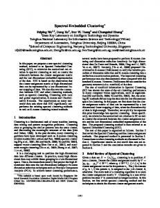
DEC-DA
𝑥
𝑧
Encoder
𝐿𝑐
Embedded feature
𝐿𝑟 Recons truction
Clustering
Decoder 𝐿 = 𝛼𝐿𝑟 + 𝛽𝐿𝑐
Figure 1: The framework of deep embedded clustering (DEC) family. The clustering loss Lc encourages the encoder to learn embedded features that are suitable for clustering task. The reconstruction loss Lr makes sure the embedded features preserve the structure of data generating distribution.
2.2. Deep Embedded Clustering Deep Embedded Clustering algorithm is first proposed by Xie et al. (2016) and further improved in various aspects by Guo et al. (2017); Dizaji et al. (2017); Li et al. (2017). To facilitate the description, in this paper, we use DEC (without a reference appended) to represent the family of algorithms that perform clustering on the embedded features of an autoencoder. A specific member of DEC family is represented by NAME-[reference]. For example, the vanilla DEC proposed by Xie et al. (2016) is referred to as DEC Xie et al. (2016), and the IDEC method proposed by Guo et al. (2017), as another member of DEC family, is represented by IDEC Guo et al. (2017). We give the framework of DEC family as in Figure 1. The objective is to minimize the following loss function: L = αLr + βLc , (2) where Lr is the reconstruction loss of an autoencoder, Lc is some kind of clustering loss, and (α, β) are coefficients to balance these two loss functions. Given a set of training samples X={xi ∈ RD }ni=1 , where D and n are the dimension and number of samples, the reconstruction loss is defined by Mean of Square Errors (MSE): n
Lr =
1X kxi − gU (fW (xi ))k22 , n i=1
where fW and gU are encoder and decoder, respectively.
3
(3)
Table 1: Configuration of DEC algorithms. “Conv” indicates whether to use convolutional networks. ∗ Note that DEPICT also incorporates the reconstruction loss between internal layers.
DEC Xie et al. (2016) IDEC Guo et al. (2017) DCN Yang et al. (2017) DBC Li et al. (2017) DEPICT Dizaji et al. (2017)
Conv No No No Yes Yes
Lr No (3) (3) (3) (3)∗
Lc (5) (5) (4) (5) (5)
The clustering loss, however, can be varied among family members. It can be the k-means loss Yang et al. (2017): n 1X Lc = kfW (xi ) − Msi k22 , (4) n i=1
where si ∈ {0, 1}K , 1> si = 1, is the cluster assignment indicator for xi , and M = [µ1 , µ2 , . . . , µK ] ∈ Rd×K contains K cluster centers in embedded feature space with dimension d. The clustering loss can also be the KullbackLeibler (KL) divergence Xie et al. (2016); Li et al. (2017); Guo et al. (2017); Dizaji et al. (2017): XX pij , (5) Lc = KL(P kQ) = pij log qij i
j
where qij is the similarity between embedded point zi and cluster center µj measured by Student’s t-distribution Maaten and Hinton (2008): (1 + kzi − µj k2 )−1 . qij = P 2 −1 j (1 + kzi − µj k )
(6)
And pij in (5) is the target distribution defined as P 2/ qij i qij � pij = P � P 2/ q q ij i j ij
(7)
DEC algorithms consist of two stages: pretraining and finetuning. The pretraining (set α = 1 and β = 0) learns valid features which are utilized to initialize the cluster centers. In the finetuning stage (set β 6= 0), clustering and feature learning are jointly performed. In this way, the learned feature will be task specific, i.e., suitable for clustering task. We summarize existing DEC algorithms in Table 1 according to the type of neural network, reconstruction loss, and clustering loss they use during finetuning. Though demonstrating promising performance, existing DEC algorithms overlook the data augmentation which has been widely used in supervised deep learning. We will fill this gap by proposing the framework of DEC with data augmentation (DEC-DA).
3. Deep Embedded Clustering with Data Augmentation As described in the last section, DEC algorithms consist of two stages: pretraining an autoencoder by reconstruction and finetuning the network by (adding) a clustering loss. We propose to incorporate data augmentation into both stages, termed DEC-DA. 4
DEC-DA
3.1. Autoencoder with Data Augmentation Data augmentation, such as random rotation, shifting, and cropping, is used as a regularization in supervised neural networks to improve the generalization. Introducing data augmentation into unsupervised learning models like autoencoders is straightforward. Given a set of training samples X = {xi ∈ RD }ni=1 , where D and n are the dimension and number of samples. For each sample xi , a random transformation Trandom is applied to get the augmented version x˜i = Trandom (xi ). Then the loss function is n
Lr =
1X k˜ xi − gU (fW (˜ xi ))k22 , n
(8)
i=1
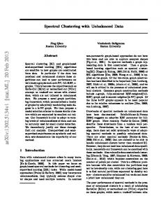
where fW and gU are encoder and decoder, respectively. By contrast with denoising autoencoder (1), we do not expect to reconstruct x from its augmented version x ˜. This is due to the fact that augmented samples share the same manifold with original samples. Ideally, the manifold learned by using augmented samples should be more continuous and smooth than that learned by using original samples. That is to say, incorporating data augmentation can help the autoencoder learn more representative features. We also do not augment input samples by adding random noise, because the samples corrupted by noise is intrinsically away from the manifold. It will be challenging to learn the real manifold from these samples with noise. 3.2. Finetuning with Data Augmentation We propose the framework of DEC-DA for the finetuning stage as illustrated in Figure 2. The loss function is L = αLr + βLc , (9) where the reconstruction loss Lr is defined by (8) and clustering loss Lc is k-means (4) or KL divergence (5). The clustering losses (4) and (5) can be abstracted into the distance between the output y and target t of the network for feature learning: Lc = dist(y, t).
(10)
In our proposed framework, the target t is computed by using clean sample x and the output y is calculated by augmented sample x ˜. The reasons are as follows. After pretraining the autoencoder, the initial features of all samples can be extracted from the embedded layer. Then we need to compute the clustering loss Lc which is used to do clustering and feature learning alternatively. When we optimize Lc with regard to network parameters, the target t will be fixed as constant. This can be regarded as supervised learning, which is supposed to benefit from data augmentation. So we calculate the output y in (10) using augmented sample x ˜. But when the network parameters are fixed, should we update the target t by using the augmented sample, too? In supervised learning, the target t is provided along with the training sample, dominating the learning process. While in our problem, we can’t get access to the “true” target and can only construct a relatively reliable “pseudo” target. In existing DEC algorithms, the target t for each sample can be regarded as the center of the cluster the sample belongs to. That is to say, the target t depends on the cluster assignment. To make sure the reliability of target t, we should use the original samples instead of augmented ones to update the cluster assignment. Furthermore, 5
Encoder 𝑓𝑊
Target
𝑧
𝑥 Clean input
𝑦
𝑡
Share weights
Augmented
𝑥
Encoder 𝑓𝑊
𝑧
𝐿𝑐 𝑦
𝐿𝑟 Decoder 𝑔𝑈
𝐿 = 𝛼𝐿𝑟 + 𝛽𝐿𝑐 Figure 2: The framework of our deep embedded clustering with data augmentation (DEC-DA). The encoder and decoder can be fully connected networks or convolutional networks. The y and t are the output and target of the feature learning model. The dashed line indicates the gradient flow. The encoder at top is only used to supply the target t and thus there’s no gradient flowing through it.
6
DEC-DA
in clustering, we only care about the cluster assignments for the given samples. Deploying data augmentation during feature learning is also to facilitate the cluster assignment. Beside Figure 2, the framework of DEC-DA is also summarized as in Algorithm 1. Algorithm 1 Deep Embedded Clustering with Data Augmentation (DEC-DA) Input: Data X; Transformation Trandom ; Number of clusters K; Output: Cluster assignment s. ˜ = Trandom (X); 1: Pretrain the autoencoder by (8) with X 2: Initialize cluster centers, s, and target t; 3: while Stopping criterion not met do ˜ and fixed t; 4: Update network by (9) with X 5: Update s and t by (10) with network (i.e. y) fixed; 6: end while
3.3. Instantiation and Implementation To validate the effectiveness of our DEC-DA, we instantiate five algorithms based on vanilla DEC Xie et al. (2016), Improved DEC (IDEC) Guo et al. (2017), and Deep Clustering Network (DCN) Yang et al. (2017). The loss functions used for pretraining and finetuning are (8) and (4) respectively. We only need to instantiate (10) for finetuning stage. By taking the algorithm based on DCN Yang et al. (2017) as an example, the objective for feature learning is ! n 1X 2 min αLr + β kfW (˜ xi ) − Msi k2 , (11) W,U n i=1
and the objective for clustering step is n
M,s
1X kfW (xi ) − Msi k22 , n
s.t.
si ∈ {0, 1}K , 1> si = 1.
min
i=1
(12)
Since we have reimplemented all algorithms under the united framework, we use new names to distinguish them from vanilla algorithms. We denote the algorithm that uses fully connected networks as Fc[*], and that uses convolutional networks as Conv[*] where “[*]” can be one of “DEC”, “IDEC”, and “DCN”. When the data augmentation is incorporated into these algorithms, we add a suffix “-DA” to their names. All algorithms with “-DA” share the identical settings with their counterpart. E.g., the only difference between FcDEC-DA and FcDEC is whether to use data augmentation during training. For all algorithms with suffix ‘-DA‘, we use the same transformation function Trandom to perform data augmentation: random shifting for up to 3 pixels in each direction and random rotation for up to 10◦ . For all Fc[*] algorithms, the autoencoder is composed of eight layers with dimensions D − 500 − 500 − 2000 − 10 − 2000 − 500 − 500 − D, where D is the dimension of input samples. Except for the input, embedded, and output layers, all internal layers are activated by ReLU Glorot
7
et al. (2011). During the pretraining stage, the autoencoder is trained in an end-to-end manner for 500 epochs by using the SGD optimizer with learning rate (lr) 1.0 and momentum 0.9. For all Conv[*] algorithms, the encoder network structure is Conv532 → Conv564 → Conv3128 → Fc10 where Convkn denotes a convolutional layer with n filters (channels), kernel size of k × k and stride of 2 as default. The decoder is a mirror of the encoder. Except for the input, embedded, and output layers, all internal layers are activated by ReLU Glorot et al. (2011). The autoencoder is pretrained end-to-end for 500 epochs using Adam Kingma and Ba (2014) with default parameters in Keras Chollet et al. (2015). Then it is finely tuned for 20,000 iterations with batch size 256 using Adam with default parameters. Other specific settings for each algorithm are as follows: • FcDEC(-DA): Set α = 0, β = 1, and optimizer SGD with lr 0.01 and momentum 0.9 for finetuning. • ConvDEC(-DA): Use convolutional autoencoder. • FcIDEC(-DA): Set α = 1, β = 0.1, and optimizer SGD with lr 1.0 and momentum 0.9 for finetuning. • ConvIDEC(-DA): Use convolutional autoencoder. • FcDCN(-DA): Set α = 0, β = 1, and optimizer Adam with lr 0.0001 during finetuning. Our implementation is based on Python and Keras Chollet et al. (2015). The source code is publicly available at Not given due to blind review protocol
4. Experiment 4.1. Experiment Settings Datasets: We conduct experiments on four image datasets as follows. • MNIST-full: A dataset consisting of 10 handwritten digits LeCun et al. (1998), total 70,000 samples. Each sample is a 28x28 gray image. • MNIST-test: A dataset that only contains the test set of MNIST-full, with 10,000 samples. • USPS1 : A dataset contains 9298 gray digit images with size of 16x16. • Fashion: A dataset of Zalando’s article images, consisting of 70,000 examples each of which is a 28x28 gray image, divided into 10 classes Xiao et al. (2017). All datasets are normalized by rescaling the elements to [0,1]. For algorithms that use fully connected networks, each sample is simply reshaped to a vector before fed into the network. Baseline methods: The proposed DEC-DA is compared with both conventional shallow clustering algorithms and state-of-the-art deep clustering algorithms. Shallow ones include k-means MacQueen (1967), normalized-cut spectral clustering (SC-Ncut) Shi and Malik (2000), large-scale spectral clustering (SC-LS) Chen and Cai (2011), locality preserving non-negative matrix factorization 1. http://www.cad.zju.edu.cn/home/dengcai/Data/MLData.html
8
DEC-DA
Table 2: Performances of DEC and DEC-DA algorithms. “Conv”, “Aug-ae”, and “Aug-cluster” denote whether to use convolutional networks, to use data augmentation during pretraining, and to use data augmentation during finetuning, respectively. Employing data augmentation in both stages leads to the best performance in most cases.
FcDEC – – FcDEC-DA ConvDEC – – ConvDEC-DA FcIDEC – – FcIDEC-DA ConvIDEC – – ConvIDEC-DA FcDCN – – FcDCN-DA
Conv
Aug-ae
Aug-cluster
× × × × X X X X × × × × X X X X × × × ×
× × X X × × X X × × X X × × X X × × X X
× X × X × X × X × X × X × X × X × X × X
MNIST-full ACC NMI 0.916 0.875 0.981 0.947 0.979 0.945 0.985 0.959 0.900 0.888 0.979 0.948 0.955 0.921 0.985 0.960 0.912 0.872 0.961 0.941 0.976 0.939 0.986 0.962 0.901 0.891 0.977 0.944 0.971 0.939 0.983 0.955 0.901 0.849 0.945 0.937 0.973 0.932 0.986 0.962
9
MNIST-test ACC NMI 0.795 0.752 0.940 0.922 0.953 0.900 0.979 0.945 0.858 0.845 0.957 0.927 0.924 0.907 0.983 0.958 0.786 0.728 0.922 0.907 0.952 0.894 0.981 0.950 0.860 0.847 0.948 0.926 0.921 0.906 0.979 0.950 0.727 0.687 0.489 0.688 0.921 0.859 0.961 0.920
USPS ACC NMI 0.763 0.784 0.830 0.885 0.960 0.904 0.980 0.945 0.786 0.822 0.830 0.902 0.965 0.919 0.987 0.962 0.771 0.799 0.823 0.884 0.967 0.918 0.984 0.954 0.792 0.827 0.823 0.906 0.917 0.902 0.984 0.955 0.699 0.722 0.685 0.771 0.951 0.895 0.969 0.929
Fashion ACC NMI 0.572 0.636 0.564 0.649 0.577 0.646 0.577 0.652 0.566 0.614 0.586 0.641 0.582 0.628 0.586 0.636 0.594 0.634 0.578 0.651 0.576 0.645 0.580 0.652 0.570 0.621 0.593 0.644 0.589 0.639 0.584 0.638 0.557 0.638 0.574 0.644 0.575 0.640 0.580 0.650
(NMF-LP) Cai et al. (2009), zeta function based agglomerative clustering (AC-Zell) Zhao and Tang (2008), graph degree linkage-based agglomerative clustering (AC-GDL) Zhang et al. (2012), and robust continuous clustering (RCC) Shah and Koltun (2017). Deep clustering algorithms include deep clustering networks (DCN) Yang et al. (2017), deep embedded clustering (DEC) Xie et al. (2016), improved deep embedded clustering with locality preservation (IDEC) Guo et al. (2017), cascaded subspace clustering (CSC) Peng et al. (2017), variational deep embedding (VaDE Jiang et al. (2017)), joint unsupervised learning (JULE) Yang et al. (2016), deep embedded regularized clustering (DEPICT) Dizaji et al. (2017), discriminatively boosted clustering (DBC) Li et al. (2017), and deep adaptive clustering (DAC) Chang et al. (2017). We report the results by excerpting from the corresponding papers or by running their released code when available. Our five algorithms FcDEC-DA, ConvDEC-DA, FcIDEC-DA, ConvIDEC-DA, and FcDCN-DA are both included into comparison. We report the result by averaging over five trials for each algorithm on each dataset. Evaluation metrics: We evaluate all clustering methods with the following metrics: clustering ACCuracy (ACC), Normalized Mutual Information (NMI). The larger value corresponds to the better clustering performance. 4.2. Effectiveness of Data Augmentation To validate the effectiveness of incorporating data augmentation, we compare the clustering performances of algorithms with and without data augmentation. The results are shown in Table 2. We can see that algorithms with “-DA” outperforms their counterparts (without “-DA”) by a large margin. For example, the ACC and NMI of FcDEC-DA algorithm on MNIST-test and USPS increase by almost 0.2, compared to FcDEC. Even on the difficult Fashion dataset, the improvement is still observable. We observed that there are very limited variations regarding shifting and rotation in Fashion dataset. This enlightens us that designing dataset specific data augmentation probably further increases the clustering performance. But in practice, to explore the variations of a given dataset is tedious. We’ll study this in future work. We have also conducted ablation study to see the effect of data augmentation in different stages. “Aug-ae” and “Aug-cluster” in Table 2 indicate whether to use data augmentation in the pretraining and finetuning stage, respectively. As we can see, data augmentation in each stage can improve the performance. So it can be applied on a single stage if it’s not convenient to apply on both stages. One exception is FcDCN without Aug-ae and with Aug-cluster on MNIST-test dataset, where the ACC drops dramatically. It may be due to that the loss function (11) fell into the degenerate solution. But we can still conclude that data augmentation in both stages can favor the clustering task. 4.3. Comparison with State-of-the-art Methods We also compare our DEC-DA algorithms with state-of-the-art clustering methods. As shown in Table 3, shallow clustering algorithms like k-means, spectral clustering, and agglomerative clustering perform worse than deep clustering algorithms in most cases. The algorithms using fully connected networks (from DCN Yang et al. (2017) to VaDE Jiang et al. (2017)) are overpowered by that using convolutional networks (from JULE Yang et al. (2016) to DAC Chang et al. (2017)). Our DEC-DA algorithms achieve the best performances on all datasets. With data augmentation, the fully connected variants can be comparable to the convolutional variants. Actually, except for FcDEC-DA on
10
DEC-DA
Table 3: Clustering performances of different algorithms in terms of ACC and NMI. All results of baseline algorithms are reported by running their released code except the ones marked by (∗) on top which are excerpted from the corresponding paper. The mark “–” denotes that the result is unavailable from the paper or the code.
k-means MacQueen (1967) SC-Ncut Shi and Malik (2000) SC-LS Chen and Cai (2011) NMF-LP Cai et al. (2009) AC-Zell Zhao and Tang (2008) AC-GDL Zhang et al. (2012) RCC Shah and Koltun (2017) DCN Yang et al. (2017) DEC Xie et al. (2016) IDEC Guo et al. (2017) CSC Peng et al. (2017) VaDE Jiang et al. (2017) JULE Yang et al. (2016) DEPICT Dizaji et al. (2017) DBC Li et al. (2017) DAC Chang et al. (2017) FcDEC-DA ConvDEC-DA FcIDEC-DA ConvIDEC-DA FcDCN-DA
MNIST-full ACC NMI 0.532 0.500 0.656 0.731 0.714 0.706 0.471 0.452 0.113 0.017 0.113 0.017 – 0.893∗ 0.830∗ 0.810∗ 0.863 0.834 0.881∗ 0.867∗ 0.872∗ 0.755∗ 0.945 0.876 0.964∗ 0.913∗ 0.965∗ 0.917∗ 0.964∗ 0.917∗ 0.978∗ 0.935∗ 0.985 0.959 0.985 0.960 0.986 0.962 0.983 0.955 0.986 0.962
MNIST-test ACC NMI 0.546 0.501 0.660 0.704 0.740 0.756 0.479 0.467 0.810 0.693 0.933 0.864 – – 0.802 0.786 0.856 0.830 0.846 0.802 0.865∗ 0.733∗ 0.287 0.287 0.961∗ 0.915∗ 0.963∗ 0.915∗ – – – – 0.979 0.945 0.983 0.958 0.981 0.950 0.979 0.950 0.961 0.920
11
USPS ACC NMI 0.668 0.627 0.649 0.794 0.746 0.755 0.652 0.693 0.657 0.798 0.725 0.825 – – 0.688 0.683 0.762 0.767 0.761∗ 0.785∗ – – 0.566 0.512 0.950 0.913 0.899 0.906 – – – – 0.980 0.945 0.987 0.962 0.984 0.954 0.984 0.955 0.969 0.929
Fashion ACC NMI 0.474 0.512 0.508 0.575 0.496 0.497 0.434 0.425 0.100 0.010 0.112 0.010 – – 0.501 0.558 0.518 0.546 529 0.557 – – 0.578 0.630 0.563 0.608 0.392 0.392 – – – – 0.577 0.652 0.586 0.636 0.580 0.652 0.584 0.638 0.580 0.650
Figure 3: Sensitivity analysis for the transformations (rotation and shifting) used in data augmentation on MNIST-test.
Fashion and FcDCN-DA on MNIST-test in terms of ACC, all of DEC-DA algorithms outperform the state-of-the-art methods by a large margin. In Table 4, we report the running time of different algorithms. All experiments are performed on a PC with Intel Core i7-6700 CPU @ 4.00GHz and a single NVIDIA GTX 1080 GPU. As it shows, RCC Shah and Koltun (2017) is the most efficient algorithm, but the performance (NMI) is inferior to ours (0.893 vs. 0.962 on MNIST-full). JULE Yang et al. (2016) and DEPICT Dizaji et al. (2017) paid a lot of time to get good results. By contrast, our DEC-DA algorithms are quite efficient to get the state-of-the-art clustering performance. By comparing algorithm X and X-DA where X can be one of FcDEC, ConvDEC, FcIDEC, ConvIDEC, and FcDCN, the extra time spent on data augmentation is acceptable. In fact, we can use multiprocessing carefully to perform data augmentation in real time. So we believe the efficiency of our DEC-DA algorithms is not a problem. 4.4. Sensitivity Analysis By regarding the transformations used for augmenting data as hyper-parameters, we can study the sensitivity. In our experiment, only random rotation and shifting are used. We sample 0◦ , 10◦ , . . . , 60◦ for rotation, and 0, 1, . . . , 6 for shifting transformation. Then on each of the resulting 49 grids, we run our FcDEC-DA algorithm on MNIST-test dataset twice. Due to limited space and computing resource, we can not show the results of all DEC-DA algorithms on all datasets. The performance in terms of NMI is reported in Figure 3. As can be seen, our FcDEC-DA outperforms the baseline FcDEC (0.75) for a wide range. When shifting for up to 6 pixels, the performance of our algorithm
12
DEC-DA
Table 4: Running time of different algorithms on MNIST-full dataset. X(-DA) = t1 (t2 ) means the running time of algorithm X is t1 and X-DA is t2 , where X can be FcDEC et.al. Algorithm RCC IDEC VaDE JULE DEPICT
Time (s) 200 1,400 3,000 20,000 9,000
Algorithm FcDEC(-DA) ConvDEC(-DA) FcIDEC(-DA) ConvIDEC(-DA) FcDCN(-DA)
Time (s) 600 (1,100) 1,700 (2,100) 700 (1,300) 2,200 (2,500) 550 (750)
drops dramatically. This is not a surprise because there will be a lot of information lost in this case. In the range of [0◦ , 40◦ ] for rotation and [1, 4] for shifting, our FcDEC-DA performs stably well.
5. Conclusion In this paper, we proposed the framework of DEC-DA by incorporating data augmentation into deep embedded clustering (DEC) algorithms. Our DEC-DA utilizes data augmentation in both pretraining and finetuning stages of DEC. Then we instantiated and implemented five DEC-DA algorithms. By comparing with state-of-the-art clustering methods on four image datasets, our DEC-DA algorithms achieved the best clustering performance. The results validate that incorporating data augmentation can improve the clustering performance by a large margin. We will explore the effect of data augmentation on other deep clustering algorithms.
References Christopher M Bishop. Pattern Recognition and Machine Learning. Springer, 2006. Deng Cai, Xiaofei He, Xuanhui Wang, Hujun Bao, and Jiawei Han. Locality preserving nonnegative matrix factorization. In IJCAI, pages 1010–1015, 2009. Jianlong Chang, Lingfeng Wang, Gaofeng Meng, Shiming Xiang, and Chunhong Pan. Deep adaptive image clustering. In ICCV, pages 5880–5888, 2017. Xinlei Chen and Deng Cai. Large scale spectral clustering with landmark-based representation. In AAAI, pages 313–318, 2011. Franc¸ois Chollet et al. Keras. https://github.com/fchollet/keras, 2015. Kamran Ghasedi Dizaji, Amirhossein Herandi, and Heng Huang. Deep clustering via joint convolutional autoencoder embedding and relative entropy minimization. In ICCV, pages 5747–5756, 2017. Xavier Glorot, Antoine Bordes, and Yoshua Bengio. Deep sparse rectifier neural networks. Journal of Machine Learning Research, 15:315–323, 2011. Xifeng Guo, Long Gao, Xinwang Liu, and Jianping Yin. Improved deep embedded clustering with local structure preservation. In IJCAI, pages 1753–1759, 2017. 13
Zhuxi Jiang, Yin Zheng, Huachun Tan, Bangsheng Tang, and Hanning Zhou. Variational deep embedding: An unsupervised and generative approach to clustering. In IJCAI, pages 1965–1972, 2017. Diederik Kingma and Jimmy Ba. Adam: A method for stochastic optimization. arXiv preprint arXiv:1412.6980, 2014. Yann LeCun, L´eon Bottou, Yoshua Bengio, and Patrick Haffner. Gradient-based learning applied to document recognition. Proceedings of the IEEE, 86(11):2278–2324, 1998. Fengfu Li, Hong Qiao, Bo Zhang, and Xuanyang Xi. Discriminatively boosted image clustering with fully convolutional auto-encoders. CoRR, abs/1703.07980, 2017. Xinwang Liu, Yong Dou, Jianping Yin, Lei Wang, and En Zhu. Multiple kernel k-means clustering with matrix-induced regularization. In AAAI, pages 1888–1894, 2016. Laurens van der Maaten and Geoffrey Hinton. Visualizing data using t-sne. Journal of Machine Learning Research, 9(Nov):2579–2605, 2008. James MacQueen. Some methods for classification and analysis of multivariate observations. In Berkeley Symposium on Mathematical Statistics and Probability, volume 1, pages 281–297. Oakland, CA, USA., 1967. Erxue Min, Xifeng Guo, Qiang Liu, Gen Zhang, Jianjing Cui, and Jun Long. A survey of clustering with deep learning: From the perspective of network architecture. IEEE Access, 2018. doi: 10.1109/ACCESS.2018.2855437. Andrew Y Ng, Michael I Jordan, and Yair Weiss. On spectral clustering: Analysis and an algorithm. In NIPS, pages 849–856, 2002. Xi Peng, Jiashi Feng, Jiwen Lu, Wei-Yun Yau, and Zhang Yi. Cascade subspace clustering. In AAAI, pages 2478–2484, 2017. Sohil Shah and Vladlen Koltun. Robust continuous clustering. Proceedings of the National Academy of Sciences of the United States of America, 114(37):9814–9819, 2017. Jianbo Shi and Jitendra Malik. Normalized cuts and image segmentation. IEEE Transactions on Pattern Analysis & Machine Intelligence, 22(8):888–905, 2000. Pascal Vincent, Hugo Larochelle, Yoshua Bengio, and Pierre Antoine Manzagol. Extracting and composing robust features with denoising autoencoders. In ICML, pages 1096–1103, 2008. Han Xiao, Kashif Rasul, and Roland Vollgraf. Fashion-mnist: a novel image dataset for benchmarking machine learning algorithms, 2017. Junyuan Xie, Ross Girshick, and Ali Farhadi. Unsupervised deep embedding for clustering analysis. In ICML, pages 478–487, 2016. Bo Yang, Xiao Fu, Nicholas D Sidiropoulos, and Mingyi Hong. Towards k-means-friendly spaces: Simultaneous deep learning and clustering. In ICML, volume 70, pages 3861–3870, 2017. 14
DEC-DA
Jianwei Yang, Devi Parikh, and Dhruv Batra. Joint unsupervised learning of deep representations and image clusters. In CVPR, pages 5147–5156, 2016. Wei Zhang, Xiaogang Wang, Deli Zhao, and Xiaoou Tang. Graph degree linkage: Agglomerative clustering on a directed graph. In ECCV, pages 428–441, 2012. Deli Zhao and Xiaoou Tang. Cyclizing clusters via zeta function of a graph. In NIPS, pages 1953– 1960, 2008.
15