DIRECT: Deep Discriminative Embedding for Clustering of LIGO Data

DIRECT: DEEP DISCRIMINATIVE EMBEDDING FOR CLUSTERING OF LIGO DATA S. Bahaadini? , V. Noroozi?? , N. Rohani? , S. Coughlin† , M. Zevin† , and A. Katsaggelos?

arXiv:1805.02296v1 [cs.LG] 7 May 2018

? Electrical Engineering and Computer Science, Northwestern University, Evanston, IL, USA ?? Department of Computer Science, University of Illinois at Chicago, IL, USA, † Center for Interdisciplinary Exploration and Research in Astrophysics (CIERA) and Dept. of Physics and Astronomy, Northwestern University, Evanston, IL, USA ABSTRACT In this paper, benefiting from the strong ability of deep neural network in estimating non-linear functions, we propose a discriminative embedding function to be used as a feature extractor for clustering tasks. The trained embedding function transfers knowledge from the domain of a labeled set of morphologically-distinct images, known as classes, to a new domain within which new classes can potentially be isolated and identified. Our target application in this paper is the Gravity Spy Project, which is an effort to characterize transient, non-Gaussian noise present in data from the Advanced Laser Interferometer Gravitational-wave Observatory, or LIGO. Accumulating large, labeled sets of noise features and identifying of new classes of noise lead to a better understanding of their origin, which makes their removal from the data and/or detectors possible. Index Terms— Deep Learning, Image Clustering, LIGO, Domain adaptation 1. INTRODUCTION The advanced Laser Interferometer Gravitational-wave Observatory (LIGO, [1]) recently made the first direct observations of gravitational waves emanating from the final orbits and merger of binary compact object systems [2, 3, 4, 5]. These observations require sensitivity to fractional changes of distance on the order of 10−21 . Though all sensitive components of LIGO are exquisitely isolated from nongravitational-wave disturbances, the extreme sensitivity of LIGO still makes it susceptible to disturbances that cause noise in the detectors and can afflict searches for gravitational waves. Transient, non-Gaussian noise sources known colloquially as glitches occur at a significant rate, come in many morphologies, and can mask or mimic gravitational-wave signals. A comprehensive classification and characterization of these noise features is needed to identify their origin, construct vetoes to eliminate them from the data, and/or to remove their root cause from the instrument itself. The Gravity Spy project [6] is designed to classify these glitches into morphological categories by combining the

strengths of machine learning algorithms and crowdsourcing. The dataset of glitches [7] are represented as spectrogram images in time-frequency-energy space, where 22 morphologically-distinct classes are currently accounted for [6]. In [7, 6, 8, 9], this multi-class classification problem has been tackled by the application of deep learning algorithms. In [9], some initial efforts toward glitch clustering are presented. Because of variable environmental conditions at the sites and changes in the sensitivity and design of the LIGO detectors over time, glitch classes are not static, and new morphological classes regularly appear in the data. Therefore, the identification of new glitch classes is a route worthy of investigation. By considering the morphological characteristics of glitches, new classes can be defined and integrated into the Gravity Spy project [6] which will bolster the number of labeled glitches in these new morphological classes. Updating glitch classes in such a manner will help us follow changes in the noise present in LIGO data and allow for their suppression or removal. In this paper, we present our model for clustering the glitches that are identified through the Gravity Spy framework as not belonging to the set of known glitch classes. Our suggested algorithm transfers knowledge from the domain of known glitch classes to the domain of unknown glitch classes. To this end, a deep neural network model is trained with the samples from known glitch classes. This neural network learns the parameters of a nonlinear embedding function that works as a feature extractor to give us a discriminative feature space where samples from the same class are close to each other while samples from different classes are far from each other. The embedding function projects samples to a discriminative space that allows the clustering algorithm to work more effectively. This enables the clustering algorithm to find potential new glitch classes over the space of unknown glitch samples. 2. PROPOSED FRAMEWORK The clustering task is an unsupervised machine learning algorithm [10]. In this study, we transfer and inject knowledge

output Objective Function Layer

fθ

fθ

CNN

θ

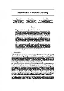
function modeled by a convolutional neural network in Fig. 1, dist is a distance function (such as Euclidean or Cosine), and m is the margin that is used to bound the distance between the items of pairs from different classes. This objective function was originally proposed in [12] for signature verification and its semi-supervised version has been proposed in [13].

CNN

2.2. DIRECT

x2

x1

Fig. 1: The schematic representation of the deep neural network that is trained to yield a discriminative feature space. CNN is the convolutional neural network. to the clustering algorithm using deep neural networks. Our algorithm, which is called Deep DIscRiminative Embedding for Clustering of LIGO Data (DIRECT), uses a labeled set of glitch classes as the source domain and a pool of unlabeled glitch samples as the target domain, which may or may not belong to the glitch classes accounted for in Gravity Spy. This type of task is also referred to as domain adaptation [11]. We define a nonlinear embedding function fθ , which is used to give a new discriminative representation for glitch data. A deep neural network model is implemented to learn fθ . The schematic representation of this model is shown in Fig. 1. The model is trained with the pairs of samples selected from the set of known glitch classes. It is trained such that in this new feature space, samples from the same class are located close to each other while samples from different classes are far from each other. This is a desirable property which is a called discriminative feature space. We hypothesize that this discriminative space, though trained with samples that may be quite different from the unlabeled samples, will lead to the improved clustering of the unlabeled testing samples. We test this hypothesis in Section 3, and the objective function which determines this discriminative space is discussed in the following section. 2.1. Objective Function The objective function L of the model is defined as L=

N X

l(y i , xi1 , xi2 ) =

i=1

N X

y i × dist(fθ (xi1 ) − fθ (xi2 ))

i=1

As DIRECT contains a deep neural network, we first train the network with a training set consisting of pairs of known sam-
ples. Given |X| labeled glitch samples, we can make |X| 2 pairs. Our labeled set of ∼10,000 images thus leads to almost 50 million pairs. To limit computational costs, we consider a smaller subset of pairs for training. In order to span the whole space of possible pairs better, for each epoch in the algorithm randomly choose a new set of pairs. There exits many optimization techniques The RMSprop [14] optimizer is used for optimizing Eq.1 chosen from [15, 14, 16, 17, 18]. Through training of the deep neural network, we learn the parameters of fθ (.) which is then used to project the unknown samples to the discriminative feature space. Specifically, we calculate z = fθ (x), where x ∈ IRd1 ×d2 ×3 (for which d1 and d2 are the first and second dimension of glitch images, respectively, and 3 is the RGB channel dimension) and z ∈ IRk (for which k is the size of the projected space). Thus fθ alters the dimensionality of the feature space as: IRd1 ×d2 ×3 → IRk . Then, a clustering algorithm such as k-means is employed on the new feature space. The general steps of the suggested method is summarized in Algorithm 1: Algorithm 1: Summary of DIRECT.  N Input: Training set: D = (xi1 , xi2 ) i=1 , Label set Y = {y i }N ,  i=1 M Testing set U = xm m=1 , Output: Embedding function fθ : IRd1 ×d2 ×3 → IRk ,  M Clusters label set L = cm m=1 Step1: Training deep neural network (shown in Fig. 1) with objective function Eq. 1 using RMSprop optimization method to estimate fθ (.) Step2: employing fθ on all xm ∈ U as z m = fθ (xm ) Step3: performing k-means algorithm on  M Z = z m m=1 and returning the corresponding cluster labels L return L

i

+ (1 − y ) × max(0, m − dist(fθ (xi1 ) − fθ (xi2 ))) (1) where N is the number of training pairs made from known classes, xi1 and xi2 are the first and second items of the ith pair, y i is the binary label of the ith pair which is one when the two items of the pair belong to the same class and zero when they belong to different classes, fθ (.) is the nonlinear

3. EXPERIMENT 3.1. Evaluation Measures We use two metrics to evaluate the performance of the clustering algorithm.

The first, known as the Normalized Mutual information (NMI) score, is a metric quantifying the similarity between predicted clusters versus true clusters. The NMI value lies in the range of 0 when there is no mutual information between two cluster assignments to 1 when there is perfect correlation ˆ between two sets. NMI is defined as N M I = √ I(Y;Y) ˆ , H(Y)×H(Y)

ˆ H and I are the true clusters, the predicted cluswhere Y, Y, ters, the entropy and the mutual information, respectively. The second, known as the adjusted rand score or adjusted rand index (ARI), estimates a similarity between predicted clusters versus true clusters by considering all pairs of samples and counting pairs that are assigned correctly into the same or different clusters. The Rand index (RI) [19] is de+S2 , where M is the number of elements fined as RI = S1M (2) in the test set U , S1 is the number of pairs of elements in U that are in the same subset in the true clustering assignment and the predicted clustering assignment, and S2 is the number of pairs of elements in U that are in different subsets in the true clustering assignment and in the predicted clustering assignment. The adjusted rand index is the corrected-for-chance version of RI. The adjusted rand index can yield negative values if the index is less than the expected index. The ARI is (RI−ExpectedRI ) defined as ARI = (max(RI)−Expected ). RI

3.2. Dataset We use Gravity Spy Dataset 1.0 presented and discussed in detail in [8], which uses data from the Hanford and Livingston detectors during the first and second observing runs of advanced LIGO. An earlier version of this dataset is used in [7, 6]. This dataset has 21 morphologically distinct glitch classes, and one catch-all ‘none of the above’ class. We do not use this class in our experiment as this class is ill-defined in terms of its morphological features. From the 21 distinct glitch classes, we randomly select 5 of them as the “unknown” classes. The other 16 classes are used for training DIRECT. It is important to emphasize that these two sets of classes are totally disjoint – all algorithms are trained with the samples of known glitch classes and tested on unknown classes.

Table 1: The performance comparison of DIRECT with the presented baselines. The best performances are bold for each evaluation measure. Method Original feature PCA Deep Autoencoder DIRECT (proposed model)

• Raw features: The first baseline performs the clustering task on the original feature space and evaluates how the efficiency of raw features for clustering and finding new classes.

ARI 0.1986 0.1938 0.3243 0.4550

• Principal component analysis (PCA): Principal component analysis is one of the standard dimensional reduction techniques which converts the original dataset into a dataset with linearly uncorrelated variables, known as principal components. Here, we use PCA to find the directions with the most variance in the known classes samples. We selected the first 50 principal components, which capture approximately 98% of the variance existing in the data. • Deep autoencoder: Autoencoder has been used for unsupervised representation learning. We can split the autoencoder into two parts: an encoder and a decoder. The encoder maps the input to an abstract, low-dimensional feature space, and the decoder maps the abstract feature space back to the original feature space. We use the features extracted by the encoder as our deep autoencoder comparison. The performance of these methods are compared in Table 1. As we expected, the performance of PCA and raw data are very close. This is mainly because the principal components learned on the space of known classes are not necessarily generalizable for the unknown classes space. DIRECT gives the best result, showing the ability of this model in transferring labeled data in a separate domain for the target clustering task. Although deep autoencoder shows better performance than PCA and raw feature, it still cannot use the labeled data information in the way DIRECT can as it is an unsupervised representation learning technique.

Performance

3.3. Baseline We compare the performance of our algorithm with the following baselines. The number of clusters is set equal to the number of unknown classes. Although in the real application of DIRECT we may not know the exact number of clusters beforehand, this exercise is meant to compare DIRECT against other representation algorithms and this assumption suits that purpose.

NMI 0.5131 0.5117 0.5451 0.5978

1 0.9 0.8 0.7 0.6 0.5 0.4 0.3 0.2 0.1 0

NMI ARI

50

100

200

350

500

Feature space dimension

Fig. 2: The effect of size of feature space k on DIRECT performance.

60

40

40

20

20

t-SNE dimension 2

t-SNE dimension 2

60

0

-20

-20

-40

-40

-60 -60

0

-40

-20

0

20

40

60

t-SNE dimension 1

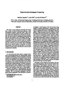
(a) Raw Feature

-60 -60

-40

-20

0

20

40

60

t-SNE dimension 1

(b) DIRECT

Fig. 3: Visualization of various feature spaces. The right plot, obtained from the proposed model, is more discriminative and many of the scattered classes seen in the raw feature space (left plot) are consolidated to form a coherent class. 3.3.1. Deep learning setting

3.4.2. Visualizing feature space

For all our deep learning implementations, we use Python utilizing the Keras library [20].

Using the t-distribution stochastic neighbor embedding (tsne) [23] algorithm, the feature space obtained from DIRECT is visualized and compared with the original feature space in Fig. 3. Examining the DIRECT feature space, we observe that samples of certain classes which are scattered in the original feature space are more tightly clustered. As an example, the two segregated clusters of the class represented by light green circles in the raw feature space (left and bottom left of the raw feature plot) are merged together as a distinct class in the feature space obtained from DIRECT space (bottom left of the DIRECT feature plot). This merging of segregated clusters can also been seen with the class represented by the small purple circles (bottom-right of raw feature plot, center-right of DIRECT feature plot). In addition to merging segregated clusters, DIRECT generally tightens the feature-space clustering of classes, as can be seen by the class represented by dark blue squares (upper-left of raw feature plot, center-right of DIRECT plot).

DIRECT configuration: For learning fθ , we first use the convolutional layers with weights of pre-trained vgg16 network [21] and add two fully connected layers with sizes of 1024 and 200 using linear and ReLU activation functions, respectively. The fully connected layer with a linear activation function has a kernel l2 regularizer of 10−4 . The objective function is given in detail in Section 2.1. The batch size is set to 20 and the number of epochs is set to 50 for DIRECT. Deep Autoencoder configuration: For deep autoencoder, we use three fully connected layer with size of 300, 200, and 300 with sigmoid activation function. The original glitch image sizes are down-sampled to 150 × 150 × 3. The objective function of the deep autoencoder is binary cross entropy. The batch size is set to 20 and the number of epochs is 50. 3.4. Model Analysis 3.4.1. Size of feature space We investigate the effect of feature space size [22] on the performance of DIRECT in Fig. 2. We see that increasing the size of k enables the algorithm to better learn the unknown sample space through learning the known sample space, but after a certain point the size of k becomes too large and DIRECT becomes prone to overfitting. We have determined that 200 dimensions is the ideal value for k, as it provides the clustering algorithm enough information. After 200 dimensions, it seems that the neural network is overfit on known classes and it may maintain noise or other irrelevant information that make the clustering less generalizable to unknown classes.

4. CONCLUSION We present a deep discriminative representation for clustering of LIGO data. A embedding function is used to transfer knowledge from a set of known glitch classes to unknown glitch classes. The parameters of this nonlinear function are learned by utilizing a deep neural network. This function maps samples to a discriminative feature space where a clustering algorithm can work more efficiently. We compare our framework with three baselines, outperforming all of them. 5. ACKNOWLEDGEMENT This work was supported in part by an NSF INSPIRE grant (award number IIS-1547880) and IDEAS Data Science Fellowship, supported by the National Science Foundation under grant DGE-1450006.

6. REFERENCES [1] LIGO Scientific Collaboration, J. Aasi, B. P. Abbott, R. Abbott, T. Abbott, M. R. Abernathy, K. Ackley, C. Adams, T. Adams, P. Addesso, and et al., “Advanced LIGO,” Classical and Quantum Gravity, vol. 32, no. 7, pp. 074001, Apr. 2015. [2] B. P. Abbott, R. Abbott, T. D. Abbott, M. R. Abernathy, F. Acernese, K. Ackley, C. Adams, T. Adams, P. Addesso, R. X. Adhikari, and et al., “Observation of Gravitational Waves from a Binary Black Hole Merger,” Physical Review Letters, vol. 116, no. 6, pp. 061102, Feb. 2016. [3] B. P. Abbott, R. Abbott, T. D. Abbott, M. R. Abernathy, F. Acernese, K. Ackley, C. Adams, T. Adams, P. Addesso, R. X. Adhikari, and et al., “GW151226: Observation of Gravitational Waves from a 22-Solar-Mass Binary Black Hole Coalescence,” Physical Review Letters, vol. 116, no. 24, pp. 241103, June 2016. [4] BP Abbott, R Abbott, TD Abbott, MR Abernathy, F Acernese, K Ackley, C Adams, T Adams, P Addesso, RX Adhikari, et al., “Binary black hole mergers in the first advanced ligo observing run,” Physical Review X, vol. 6, no. 4, pp. 041015, 2016. [5] Benjamin P Abbott, Rich Abbott, TD Abbott, Fausto Acernese, Kendall Ackley, Carl Adams, Thomas Adams, Paolo Addesso, RX Adhikari, VB Adya, et al., “Gw170817: observation of gravitational waves from a binary neutron star inspiral,” Physical Review Letters, vol. 119, no. 16, pp. 161101, 2017. [6] Michael Zevin, Scott Coughlin, Sara Bahaadini, Emre Besler, Neda Rohani, Sarah Allen, Miriam Cabero, Kevin Crowston, AK Katsaggelos, SL Larson, et al., “Gravity spy: integrating advanced ligo detector characterization, machine learning, and citizen science,” Classical and Quantum Gravity, vol. 34, no. 6, pp. 064003, 2017.

[10] Jeremy Watt, Reza Borhani, and Aggelos Katsaggelos, Machine Learning Refined: Foundations, Algorithms, and Applications, Cambridge University Press, 2016. [11] Ian Goodfellow, Yoshua Bengio, and Aaron Courville, Deep learning, MIT press, 2016. [12] Jane Bromley, Isabelle Guyon, Yann LeCun, Eduard S¨ackinger, and Roopak Shah, “Signature verification using a” siamese” time delay neural network,” in Advances in Neural Information Processing Systems, 1994, pp. 737–744. [13] Vahid Noroozi, Lei Zheng, Sara Bahaadini, Sihong Xie, and Philip S Yu, “Seven: deep semi-supervised verification networks,” in Proceedings of the 26th International Joint Conference on Artificial Intelligence. AAAI Press, 2017, pp. 2571–2577. [14] Geoffrey Hinton, Nitish Srivastava, and Kevin Swersky, “Neural networks for machine learning lecture 6a overview of mini-batch gradient descent,” 2012. [15] Matthew D Zeiler, “Adadelta: an adaptive learning rate method,” arXiv preprint arXiv:1212.5701, 2012. [16] Diederik P. Kingma and Jimmy Ba, “Adam: A method for stochastic optimization,” CoRR, vol. abs/1412.6980, 2014. [17] F. Mansoori and E. Wei, “Superlinearly convergent asynchronous distributed network newton method,” in 2017 IEEE 56th Annual Conference on Decision and Control (CDC), Dec 2017, pp. 2874–2879. [18] V. Noroozi, A. Hashemi, and M.R Meybodi, “Alpinist cellularde: a cellular based optimization algorithm for dynamic environments,” in Proceedings of the 14th annual conference companion on Genetic and evolutionary computation. ACM, 2012, pp. 1519–1520. [19] Lawrence Hubert and Phipps Arabie, “Comparing partitions,” Journal of Classification, vol. 2, no. 1, pp. 193– 218, Dec 1985.

[7] Sara Bahaadini, Neda Rohani, Scott Coughlin, Michael Zevin, Vicky Kalogera, and Aggelos K Katsaggelos, “Deep multi-view models for glitch classification,” in Acoustics, Speech and Signal Processing (ICASSP), 2017 IEEE International Conference on. IEEE, 2017.

[20] Franc¸ois Chollet et al., https://github.com/keras-team/keras, 2015.

[8] S. Bahaadini, V. Noroozi, N. Rohani, S. Coughlin, M. Zevin, J.R. Smith, V. Kalogera, and A. Katsaggelos, “Machine learning for gravity spy: Glitch classification and dataset,” Information Sciences, vol. 444, pp. 172 – 186, 2018.

[22] Yiming Yang and Jan O Pedersen, “A comparative study on feature selection in text categorization,” in International Conference on Machine Learning (ICML), 1997, vol. 97, pp. 412–420.

[9] D. George, H. Shen, and E. A. Huerta, “Glitch Classification and Clustering for LIGO with Deep Transfer Learning,” ArXiv e-prints, Nov. 2017.

“Keras,”

[21] Karen Simonyan and Andrew Zisserman, “Very deep convolutional networks for large-scale image recognition,” arXiv preprint arXiv:1409.1556, 2014.

[23] Laurens van der Maaten and Geoffrey Hinton, “Visualizing data using t-sne,” Journal of Machine Learning Research, vol. 9, no. Nov, pp. 2579–2605, 2008.