CS229,Technical Report, 2014
Deep Learning Architecture for Univariate Time Series Forecasting Dmitry Vengertsev1 Abstract This paper studies the problem of applying machine learning with deep architecture to time series forecasting. While these techniques have shown promise for modeling static data, applying them to sequential data is gaining increasing attention. This paper overviews the particular challenges present in applying Conditional Restricted Boltzmann Machines (CRBM) to univariate time-series forecasting and provides a comparison to common algorithms used for time-series prediction. 1 Department
of Computer Science Stanford University
[email protected]
1. Introduction Forecasting future values of observed time series plays an important role in nearly all fields of science and engineering, such as economics, finance, business intelligence, and industrial applications. Time series forecasting itself bares numerous complexity aspects, moreover, with the rapid growth of big data, time-series forecasting algorithms will have to analyze increasingly massive datasets. There has been extensive research on using machine learning techniques for time-series forecasting. In [1] several Machine Learning algorithms were presented to tackle timeseries forecasting problem, such as multilayer perceptron, Bayesian neural networks, K-nearest neighbor regression, support vector regression, and Gaussian processes. In [3], the effectiveness of local learning techniques is explored for dealing with temporal data. The main goal of this project is to explore the application of the novel deep learning algorithms for the problem of time series prediction. Deep architecture allows us to construct complex models that have high VC dimension and able to describe complex time series. For example, it was shown that the use of Recurrent Neural Network improve accuracy of energy load forecasting [4]. For the overview of unsupervised feature learning for time-series modeling, refer to [10]. Starting with traditional statistical approaches like AutoRegressive Integrated Moving Average (ARIMA), we further increase VC dimension of models by using Machine Learning techniques such as Multi-Layer Perceptron (MLP) and Support Vector Regresison for time series forecasting. Finally, the results of ARIMA, MLP and SV regression are compared to the case of neural network with deep architecture, Conditional Restricted Boltzmann Machine. As a benchmark dataset for testing and comparison of forecasting algorithms, we selected M3 competition dataset [8]. In particular, we consider 1428 monthly time series of
different length. Each time series is unique with 80 − 90% of datapoints marked as historical data and 10 − 20% marked as data for prediction. Data set includes several data types: demographic, finance, industrial, macro and micro economy.
2. Time Series Forecasting Starting with algorithms with lower VC dimension: ARIMA, SV regression, and MLP, we go further and apply deep architecture such as pre-training with continuous Restricted Boltzmann Machine (RBM) and Conditional RBM. 2.1 Auto Regressive Integrated Moving Average It was decided to start with statistically sophisticated model Autoregressive Integrated Moving Average algorithm (ARIMA), which is one of the traditional algorithms for time series forecasting [10]. Autoregressive models accurately predict shortterm temporal structures, but for the case of long term highlevel structures performance drops since these models assume certain stationary properties of time series. After tuning three parameters of ARIMA - number of autoregressive terms, number of nonseasonal differences needed for stationarity, and number of lagged forecast errors in the prediction equation, high prediction accuracy was obtained, Table 1. 2.2 Multilayer Perceptron and Support Vector Regression To address the drawbacks of ARIMA related to stationarity assumption, it was decided to use Machine Learning approaches. Machine Learning algorithms for time series forecasting have obtained popularity, and among the most established are Support Vector Regression and Multi-Layer Perceptron, [1], [3]. Support Vector Regression is a modification of SVM, where the hypothesis has the form hw,b (x) = wT x + b and
Deep Learning Architecture for Univariate Time Series Forecasting — 2/5
Hidden Layer
RBM:
Hidden Layer, h
Input Layer Input Layer
Output Layer Visible Layer, v
Output Layer
Hidden Layer
a.
Multi-Layer Perceptron
b.
Restricted Boltzmann Machine for Multi-Layer Perceptron
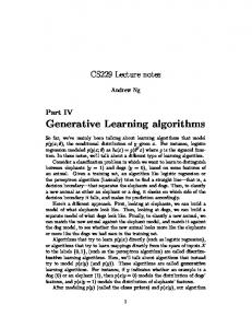
Figure 1. Network Topologies
the original margin constraint is modified to represent the distance between the continuous output of training example and our hypothesis’ output. Multi-Layer Perceptron (MLP) is a heavily parameterized feedforward neural network, Fig.1, by selecting number of hidden units the complexity of the model is controlled. For MLP and SV regression, sliding window is used to construct features from time series - the lagged time series values ut−N+1 , · · · , ut , and the value to be predicted is the next value ut+1 (for one-step ahead forecasting). In addition, smoothing window was applied to time series, to improve the model generalization, but it introduces high bias in both Support Vector Regression and Multi Layer Perceptron, so it was not used in the final results presented. For Multi-Layer Perceptron, sliding window of size N = 3 gave the model with the lowest combination of variance and bias for given number of hidden units, which is consistent with other papers where smaller sliding window shows smaller bias, Fig. 2. Table 1 summarizes performance of MLP and SV regression. Comparing to ARIMA, which underfits test data in longterm, MLP shows significant improvement, Fig.3.
Indeed, big reconstruction error from hidden units back to visible units prevented us from using it. There are possibly several reasons why pre-training with RBM did not work for time series: 1) RBM extension to continuous valued input is not appropriate and 2) dependencies between input parameters that are not modeled by RBMs. Regarding the first concern, typical RBM uses binary logistic units for visible nodes, we used the trick described in [2], where continuous-valued inputs are scaled to (0, 1) and then are treated as probability for binary random variable to take value 1. This approach worked for grayscale images [2], but for the time series forecasting it was inappropriate. Therefore, another approach described in [5] was used in the next subsection, where the noise is added to sigmoid units to handle continuous input to RBM. As for the second concern, a special form of RBM, called conditional RBM [12], that takes into account temporal dependencies was used.
2.4 Conditional Restricted Boltzmann Machines Using Conditional Restricted Boltzmann Machines that was presented by Taylor [11],[14] for human motion estimation, we are aiming to capture most temporal structures of time series and therefore enhance RBM. For more details refer to 2.3 Multi-layer Perceptron with Continuous RBM Pre- appendix A. training In CRBM, connections between current time slice vt and MLP involves random initialization of weights, therefore pre- several previous time slices vt−1 , vt−2 , · · · , vt−N+1 are contraining allows the initial weights land in a better start. Re- sidered, Fig.4. These connections correspond to autoregresstricted Boltzmann Machines (RBM) [6] can find such initial sive component and therefore model short term dependencies. weights. Fig.1-b shows the process of pre-training. For the Moreover, fixed connections from previous time slices to hidhidden layer in the MLP network, we construct an RBM that den units are added to capture long-term dependencies. In trains on the inputs given for that layer. The final weights of the Taylor’s paper, where CRBM was applied to a model of the RBM are given as the initial weights of the layer in the motion, isolated blocks of time series (mini-batches) were MLP network. used for speeding up learning. For the motion estimation, There are several examples when pre-training has shown sequential processing through the training data sequences was that RBMs can improve the final performance, for instance for unnecessary and therefore mini-batches were permuted for betMNIST digits classification. However, in the case of lagged ter learning. In our case, however, sequence of mini-batches time series features, RBM did not improve the prediction. does matter and therefore we do not perform permutation.
Deep Learning Architecture for Univariate Time Series Forecasting — 3/5
Mini-batches of size 24 were used, and the input time series were rescaled to have zero mean and unit variance. Since training and testing CRBM for 1428 monthly series takes approximately two days on high-end laptop, computational expense was a limiting factor, and therefore limited number of experiments were performed to determine parameters of the model. The best parameters from the few experiments were : delay = 12, batch size = 24, number of hidden units 300 and number of epochs 2000 (not optimal). Dependence of prediction error on number of epochs is shown at Fig.5 2.5 Conditional Restricted Boltzmann Machines - Error Analysis Performance of CRBM for time series prediction was compared to MLP performance Fig.6-a, where testing RMSE for both algorithms are shown for all time series (by time series id). For short time series, Fig.6-b, series with id from 0 to 277 that have length of around 50 (vertical blue dashed lines),have better prediction with CRBM than MLP. Also CRBM shows better performance for several time series with longer lengths, for instance id 803, Fig.6-a.mlp and Fig.6-a.crbm. Overall, by looking at Fig.6-a, even CRBM without fine tuning of parameters and pre-training is at least comparable to MLP.
Figure 3. Comparing prediction from ARIMA and MLP,
red:train, blue:test,black:ground truth Hidden Layer, h
... fixed fixed
fixed
fixed
...
Visible Layer, v
3. Results and Discussion For simplicity of comparison of algorithms RMSE metric was used, although more sophisticated metrics exist [8] to gauge accuracy of time series forecasting. Table 1 summarizes RMS error for the different algorithms. Cross validation was not performed for CRBM only due to limitation of computational resources. Note that the algorithms ARIMA, SV Regression and MLP - were severely tuned by empirical search of the best model parameters. On the other hand RMSE for Conditional RBM given above was not obtained by fine tuning, again due to limitation of computational recourses. Moreover, in order to speed up the learning, number of epochs for training of
v_{t-3}
v_{t-2}
v_{t-1}
v_{t}
Figure 4. Conditional RBM with delay of size two
CRBM was 2000 that is smaller than optimal value (close to 4000, Fig.5). There are several ways to further improve performance of CRBM for univariate time series forecasting. First, additional data cleaning can be performed to remove outliers. Second, by introducing conditional dependence of hidden units longterm structures should be captured better, though it can make training more complex. Third, stack of CRBMs can be used to add more layers and to further increase VC dimensions of hypothesis to capture more complex dependencies.
4. Conclusion Deep neural network are able to accurately predict time series. It is clear from Table 1 that Conditional Restricted Boltzmann Machines are comparable or better than our competing methods. As mentioned above, the prediction accuracy can be Table 1. Comparing CRBM to Other Models
Figure 2. RMSE of MLP depending on various sizes of sliding window
Learning Method
Train RMSE
ARIMA SV Regression MLP Conditional RBM+
552.99 592.29 604.08 707.81
Test RMSE 803.16 832.65 762.55 806.70
Deep Learning Architecture for Univariate Time Series Forecasting — 4/5
Figure 6. a. Comparison of test RMSE for MLP and CRBM; b. Length of train part of time series
Deep Learning Architecture for Univariate Time Series Forecasting — 5/5
] := B(delay) · h + hbias, where A(delay) and B(delay) hbias are weighting parameters from visible units to delayed visible units, and weights from delayed visible units to hidden units.
References [1]
Ahmed, et.al, Empirical Comparison of Machine Learning Models for Time Series Forecasting, Econometric Reviews, 29.5-6:594-621, 2010
[2]
Bengio, et.al,Greedy Layer-Wise Training of Deep Networks, Advances in Neural Information Processing Systems 19, 2007
[3]
Bontempi, et.al, Machine Learning Strategies for Time Series forecasting, Business Intelligence, Springer, 62-77, 2013
[4]
Busseti, et.al, Deep Learning for Time Series Modeling, Technical report, Stanford University, 2012
[5]
Chen, et.al, Continuous Restricted Boltzmann Machine with an Implementable Training Algorithm, Vision, Image and Signal Processing, 150.3, 2003
[6]
Hinton, et.al, Reducing the Dimensionality of Data with Neural Networks, Science, 313.5786:504-507, 2006
[7]
Hinton, et.al, Training Products of Experts by Minimizing contrastive Divergence,” Neural Computing, 14: 1771–1800, 2002
[8]
Hyndman, et.al, Another Look at Forecasting Accuracy Metrics for Intermittent Demand, International Journal of Applied Forecasting, 4,43-46, 2006
[9]
L¨angkvist, et.al, A Review of Unsupervised Feature Learning and Deep Learning for Time-Series Modeling, Pattern Recognition Letters 42:11-24, 2014
[10]
Makridakis, et.al, The M3-Competition: Results, Conclusions and Implications, International Journal of Forecasting 16.4: 451-476, 2000
[11]
Taylor, et.al, Modeling Human Motion using Binary Latent Variables, Advances in Neural Information Processing Systems, 2006
[12]
Sutskever, et.al, Learning Multilevel Distributed Representations for High-Dimensional Sequences, University of Toronto, 2006
[13]
forecasters.org/resources/time-series-data/m3competition/
Figure 5. Selecting optimal number of epochs.
improved by tuning parameters of CRBM (computationally intensive). Moreover, further improvement is possible if more complex models are used that take into account dependencies among hidden layers and by stacking Conditional RBMs. I was disappointed with the performance of Multi-Layer Perceptron with RBM pre-training, due to temporal dependencies of visual units is not considered in RBM, yet potentially with the right lagged time series as an input MLP with pretrained RBM should work. Another concern of MLP with pre-trained RBM is the way of handling continuous input, probably the Gaussian nodes with unit variance are not the best distribution to represent many datasets.
Appendix A - Energy based Models and CRBM Learning As mentioned in section 2.4, Conditional RBM is a modification of RBM with additional connections Fig.4. Conditional distributions that are used for propagation from visible units vi to hidden units h j and vise versa are given by: ^j + (v · w) j ) P(h j = 1|v) = g(hbias ^i + (h · w)i , 1), P(vi |h) = N(vbias where g is a logistic function, and N(m, σ ) is normal distribution that models continuous-valued input for RBM. Loglikelihood is given by in form of free energy: E(v, h) = −log(v, h) = ∑ i
^i )2 (vi − vbias ^j · h j − ∑ hbias 2·σ2 j
− ∑ vi h j wi j i, j
The main idea is include directed connections between visible units (data from previous time steps) into a dynami^i , and the directed connections from cally changing bias vbias ^i . previous time steps of visible units to hidden units as hbias For the learning rule we use standard update of weights and biases using contrastive divergence [7]. Update of dynamically ] := A(delay) · v + vbias and changing biases is given by: vbias
[14]
https://gist.github.com/gwtaylor/2505670