Revista Brasileira de Computação Aplicada, July, 2018
DOI: 10.5335/rbca.v10i2.7904 Vol. 10, No 2, pp. 54–63 Homepage: seer.upf.br/index.php/rbca/index
ORIGINAL PAPER
Hybrid deep learning approach for financial time series classification Carlos A. S. Assis1 , Eduardo J. Machado1 , Adriano C. M. Pereira2 and Eduardo G. Carrano2 1
Centro Federal de Educação Tecnológica de Minas Gerais and 2 Universidade Federal de Minas Gerais *
[email protected]; †
[email protected];
[email protected] [email protected]
Received: 14/02/2018. Revised: 16/06/2018. Accepted: 21/06/2018.
Abstract This paper proposes a combined approach of two machine learning techniques for financial time series classification. Boltzmann Restricted Machines (RBM) were used as the latent features extractor and Support Vector Machines (SVM) as the classifier. Tests were performed with real data of five assets from Brazilian Stock Market. The results of the combined RBM + SVM techniques showed better performance when compared to the isolated SVM, which suggests that the proposed approach can be suitable for the considered application. Key words: Restricted Boltzmann Machines. Deep Learning. Stock Market.
Resumo Este trabalho propõe uma abordagem combinada de duas técnicas de aprendizado de máquina para classificação de séries temporais financeiras. Foram utilizadas Máquinas de Boltzmann Restritas (RBM) como o extrator de características latentes e Máquinas de Vetores de Suporte (SVM) como o classificador. Cinco conjuntos de dados reais de ativos ou ações da BM&FBOVESPA foram usados para validação da abordagem. Em geral, as técnicas RBM + SVM combinadas apresentaram resultados superiores ao SVM isolado, confirmando o potencial da abordagem proposta. Palavras-Chave: Máquina de Boltzmann Restrita. Aprendizagem Profunda. Mercado de Ações.
1
Introduction
Predicting the future is certainly one of the greatest ambitions of human beings. There is no perfect system that manages to do that, but it is possible to find in the literature many attempts of doing so in several different contexts (Barrymore, John ; 2017). Considering that financial markets are environments that provide great opportunities, many studies have been developed in order to carry out predictions for this kind of application (Tkac and Verner; 2016; Cavalcante et al.; 2016). Most of these studies focus on prediction error minimization, supporting the task of predicting the best moment for buying or selling
an asset. For that, models trained with historical data are used aiming to predict future behavior. Many researchers Meesad and Rasel (2013); Nametala et al. (2016); Persio and Honchar (2016); Patel et al. (2015); Pimenta et al. (2014) have worked towards the improvement of already existing predictors. Many of these studies are based on recent machine learning techniques, such as Support Vector Machines (SVM) (Vapnik; 1995), Artificial Neural Networks (ANNs) (McCulloch and Pitts; 1943) and Genetic Programming (GP) (Koza; 1992). However, it is well known by the machine learning community that the high dimensionality of inputs usually leads to the reduction of computational performance
54
Assis et al./ Revista Brasileira de Computação Aplicada (2018), v.10, n.2, pp.54–63 |
and precision of the classification and regression results (Sá and Albertini; 2014). Theoretically, it is intuitive to think that the bigger the amount of attributes, the more information would supposedly be available for the algorithm. However, the increase in data attributes makes them tend to becoming more sparse, generating situations that considerably impair training (optimal locations of the error function, for example). This difficulty resulting from high-dimensional spaces is usually called curse of dimensionality (Liu and Motoda; 2007). In order to improve the precision of classification algorithms, it is recommended that a prior selection of features be carried out. Nevertheless, this step usually strongly depends on a specialist in the studied application. This study proposes the use of a recent artificial neural network, called Restricted Boltzmann Machine (RBM) (Hinton and Salakhutdinov; 2006), to carry out the selection of features for the later application of a machine learning technique in the prediction of financial time series (SVM). This approach of deep neural networks is a powerful tool in the area of machine learning and has been used in order to extract features, thus supporting in the reduction of dimensions and enabling the improvement of data classification (Hrasko et al.; 2015). This kind of ANN is characterized by its capacity of learning internal representations and solving complex combinatorial problems (Cai et al.; 2012). The main contribution of this work was presenting a combination of RBM and SVM machine learning techniques to predict stock market asset trends. Five real data sets of the BM&FBOVESPA were used to validate the study. Comparisons were also made between combined techniques and SVM by itself, with the proposed approach generally presenting higher accuracy. The remaining of this text is organized as follows: Section 2 describes the problem and some correlated studies; Section 3 presents a description of the RBM technique used; Section 4 describes the methodology that will be applied in Section 5, in which the results of the prediction of five real and different financial time series are presented. Finally, Section 6 presents our conclusion.
2
Problem Definition & Related Work
The base problem of this study, in general terms, is the prediction of variations in stock market asset prices. More specifically, historical data on price and volume were assessed using technical analysis (Kirkpatrick and Dahlquist; 2006) with the purpose of predicting price changes with the highest precision possible. This section presents a general view of the basic concepts of financial market and some correlated studies.
2.1
Financial Market
The financial market is the place where people can negotiate (buy or sell) assets such as real state, goods and exchange. The purpose of the market is to gather many sellers in one single place, making
55
them accessible to interested buyers. Markets are considered a vital part of any economy, since, as their movement increases, there are more opportunities for buyers to apply their resources and contribute to heating the economy (Neto; 2009). The stock exchange is the negotiation environment in which investors may buy or sell titles through direct negotiation, with or without the support of negotiation correspondents. In the case of the Brazilian stock exchange, the negotiation is done through brokers (Bússola do Investidor; 2017)1 . In Brazil, the role of the stock exchange is represented by BM&FBOVESPA (2017), who is the owner of two stock exchanges: BM&F, which focuses on the negotiation of agriculture and livestock products, and financial instruments; and BOVESPA, which focuses on the negotiation of stocks and stock options. In the stock market, the investor gains profit by buying undervalued stocks and selling them at moments of higher value. The profit of the investment is determined by the difference between the buying and the selling price, adding benefits such as dividends and discounting transaction fees (Bússola do Investidor; 2017). Usually, in order to predict if the value of a stock will increase or not, analysts use two diagnostic mechanisms, the fundamental analysis and the technical analysis (Anghel; 2013): • Fundamental Analysis: in this kind of analysis, the references for the investor are parameters that define the financial situation of the company, such as net profit, level of indebtedness and distribution of dividends, among others. In summary, the fundamental analysis assumes that stocks have an intrinsic value which would correspond to its fair price. This price, in turn, would be determined by the income stream measured for the stock and effectively distributed throughout a given period of time, discounting the present value. this analysis focuses • Technical Analysis: on information regarding stock price and buying/selling movement in a given period of time. This fact enables the projection of a trajectory or probable future changes in stock prices. Since this approach is applied in this study, it will receive greater focus. Investors who use the technical analysis seek to identify possible trends, since this analysis assumes that these trends follow a cyclical pattern (Noronha; 2003). This identification is usually based on chart patterns. After some time, these chart patterns were translated into numerical or logical indicators that facilitate the automatic processing of time series in order to identify possible opportunities. The technical analysis indicators are usually categorized as (Bússola do Investidor; 2017): • Momentum Indicators: they usually indicate the moments of entering and exiting the market (e.g., Relative Strength Index, Williams %R and Rate of Change).
1 Financial
institutions that intermediate between investors and the stock exchange.
the
negotiation
56
|
Assis et al./ Revista Brasileira de Computação Aplicada (2018), v.10, n.2, pp.54–63
• Trend Indicators: they indicate market direction – upward or downward (e.g., Moving Averages, Average Directional Index, Moving Average Convergence / Divergence). • Volatility Indicators: they show whether prices are too volatile, that is, without a defined trend (e.g., Bollinger Bands, Price Channel, Average True Range). • Volume Indicators: they are based on the fact that volume usually precedes price movement (e.g., On Balance Volume, Volume Oscillator, Chaikin Oscillator).
used a data set of the period from 1990 to 2009. The results showed that the use of RBMs enabled the reduction of input data dimensionality and the extraction of important features to support in the prediction of future prices.
Considering the innate complexity and dynamism of financial market predictions, there is a constant debate regarding the possibility of predicting stock price changes. According to Moura (2006), the traditional analysis methods (technical and fundamental) are not capable of identifying the non-linear relations between the many variables that comprise the price of a stock and its movement upwards or downwards, leading to the need of using more advanced techniques.
The next section presents the theoretical basis proposed in this study.
2.2
Related Studies
Considering the scenario of uncertainties of the stock market, many studies were or are being developed to support in the prediction of trends in this market. Nelson and Pereira (2016) applied neural networks of the type Long Short-Term Memory (LSTM) for the prediction of stock price trends. A prediction model was created and a series of experiments were carried out using assets of BM&FBOVESPA. The results found were considered satisfactory, with an average accuracy of up to 55.9% in predicting whether the price of a given stock would rise or not in the immediate future. The model was also assessed under financial perspectives, showing promising results regarding its return. Franco and Steiner (2014) compared neural networks of the types Multi Layer Perceptron (MLP), Radial Basis Function (RBF) and Layer Recurrent Network (LRN) as techniques for predicting the future value of certain stocks in BM&FBOVESPA. A total of 496 closing prices in reverse auction for four assets were used in the data set in the period ranging from February 27th, 2012, to February 25th, 2014. The accuracy measure used for validation was the mean squared error between the values predicted by the RNAs and the real values. The best prediction technique was that of LRN, with error values of the order of 10–11 . Zhu et al. (2014) implemented a decision-making support system for the buying and selling of assets. This system used Deep Belief Networks (DBN) to predict stock prices. The experiment used a set of 400 stocks from the S&P 500. This data set comprised 12 financial indicators. The authors stated that the proposed system was capable of predicting stock prices and attaining high financial performance. However, they showed that DBNs require a lot of time to be trained with historical data. For that reason, speed was an obstacle to the system. Takeuchi and Lee (2014) developed an algorithm based on Restricted Boltzmann Machines (RBM) to extract latent features of Nasdaq assets. The authors
Based on the survey by Li and Ma (2010), it is possible to observe that many studies in the literature address the theme of predicting trends in financial series but few of them use RBM. No studies could be found that combine SVM, RBM and technical analysis. Additionally, none of the studies related to RBM were applied to BM&FBOVESPA.
3
Theoretical Basis
This section addresses the main concepts required for the understanding of the proposed tool.
3.1
Restricted Boltzmann Machines (RBM)
The Restricted Boltzmann Machines (Hinton and Salakhutdinov; 2006) are unsupervised learning neural networks. They are mainly characterized by their ability to learn internal representations and to solve complex combinatorial problems. In general, the RBM is a stochastic network comprising two layers: a visible layer and a hidden layer. The layer of visible units represents the observed data and is connected to the hidden layer, which, in turn, must learn to extract features from these data. Originally, the RBM was developed for binary data, both in the visible and the hidden layers. Considering that there are problems for which it is necessary to process other data types, Hinton and Salakhutdinov (2006) proposed a Gaussian-Bernoulli RBM (CRBM), which uses normal distribution to model neurons in the visible layer. This study describes the basic concepts of the CRBM approach, considering that the inputs in this study are data of continuous type. In RBM, the connections between neurons are bidirectional and symmetrical, which means that there is information traffic in both directions of the network. Besides, in order to simplify inference procedures, neurons of the same layer are not connected between themselves. Therefore, only neurons of different layers are connected, which explains why it is called restricted. Figure 1 shows an RBM with m neurons in the visible layer (v1 , . . . , vm ), n neurons in the hidden layer (h1 , . . . , hn ), being (a1 , . . . , am ) and (b1 , . . . , bn ) the bias vectors (b) and, finally, the weight matrix of connections W. The set (W, a, b) will be called θ. The RBM is an energy-based probabilistic model. That means that the joint probability distribution of the configuration (v,h) is achieved using Equations 1 and 2:
p(v, h; θ) = P
e–E(v,h;θ) –E(v,h;θ) v,h e
(1)
Assis et al./ Revista Brasileira de Computação Aplicada (2018), v.10, n.2, pp.54–63 |
57
E D E ∂p(v, θ) D = vi hj – vi hj ∂θ d m D E D E in which the components vi hj and vi hj d
Figure 1: RBM with 4 visible units and 3 hidden units.
E(v, h; θ) = –
m n X (vi – ai )2 X – bj hj – 2 2σi i=1
j=1
i,j=1
vi h w (2) σ 2 j ij
The probability that the network attributes to a visible vector v is given by the sum of all the probabilities of the hidden vectors h, calculated by Equation 3: P –E(v,h;θ) e p(v; θ) = P h –E(v,h;θ) v,h e
(3)
As the RBM is restricted, the probability distributions of h given v and of v given h are described by Equations 4 and 5: p(h|v; θ) =
Y
p(hj |v)
(4)
are
used to represent the computed expectations about the data and the model, D respectively. E The estimation of vi hj
d
is obtained in a simple
way by means of the conditional probabilities p(hj = 1|v; θ) and Dp(vi E= v|h; θ). However, obtaining an estimate of vi hj
m,n X
m
(8)
m
is much harder. This can be done
by means of Gibbs sampling (Geman and Geman; 1984) using random data feeding the visible layer. Still, this procedure may take a lot of time to achieve an adequate result. Fortunately, a quicker procedure called contrastive divergence (CD) was proposed by Hinton (2006). The idea behind this method is to feed the visible layer with training data and execute Gibbs sampling only once, which has been called reconstruction. For the application of the CD algorithm, the first step is to match the visible layer v0 to the input data and, soon after, estimate the hidden layer h0 using the conditional probability p(hj = 1|v; θ). With that, D E vhT = v0 hT 0 . Then, based on h0 , v1 should be d
estimated using the conditional probability p(vi = v|h; θ). Similarly, based on vD is estimated, again 1 , h1 E by p(hj = 1|v; θ). With that, vhT
m
= v1 hT 1 . Finally,
the set of parameters θ are updated as follows:
j=1,...,n
Wt+1 = Wt + ∆Wt → ∆Wt p(v|h; θ) =
Y
p(vi |h)
(5)
T t t–1 = η(v0 hT 0 v1 h1 ) – ρW + α∆W
i=1,...,m
In the CRBM version (Hinton and Salakhutdinov; 2006), in which the visible layer is continuous and the hidden layer is binary, the conditional distributions are described by Equations 6 and 7:
p(hj = 1|v; θ) = φ(bj +
m X
vi wij )
(6)
hj wij , σ 2 )
(7)
i=1
p(vi = v|h; θ) = N(v|ai +
n X j=1
in which φ(x) = 1+e1 –x (logistic function) and N is a normal distribution, with mean v and standard deviation σ 2 , usually 1. The purpose of the RBM is to estimate the values of the components of vector θ that cause the energy level of the network to decrease. Since p(v; θ) is the input data distribution, θ can be estimated by the maximization of p(v, θ) or, in an equivalent manner, log p(v, θ). Therefore, the descending gradient of log p(v, θ) regarding θ is calculated by Equation 8.
at+1 = at + ∆at → ∆at = η(v0 – v1 ) + α∆at–1
bt+1 = bt + ∆bt → ∆bt = η(h0 – h1 ) + α∆bt–1 considering that (W, a, b) are randomly initialized. The pseudocode of the CD algorithm is presented as follows in Algorithm 1: The parameters η, ρ and α are known as learning rate, weight decay and momentum. Hinton (2010) suggests η = 0.01, ρ = [0.01, 0.0001] and α = 0.5 for an iteration lower than 5 and α = 0.9, in the opposite case. The RBM has four hyperparameters: the amount of neurons in the visible layer (v), the amount of neurons in the hidden layer (h), the learning rate (lr) and the amount of cycles (ep). If the learning rate is too low, network learning is too low; if it is too high, it generates oscillations in the training and prevents the convergence of the learning process. Usually, its value varies from 0.1 to 1.0. The number of cycles is the number of times in which the training set is presented to the network. An excessive number of cycles can cause the network to lose its generalization power (overfitting). On the other hand, with a
58
|
Assis et al./ Revista Brasileira de Computação Aplicada (2018), v.10, n.2, pp.54–63
Algorithm 1 Pseudocode of the algorithm: Contrastive Divergence 1: procedure CD 2: Prepare set of input data Inform the number of neurons for hidden layer 3:
h
4: 5: 6: 7: 8: 9: 10: 11: 12:
Initialize parameters η, ρ and α Randomly initialize θ while number of iterations or minimum error satisfied do Match visible layer v0 to input data; Estimate hidden layer h0 using the condit. probability p(h|v)) Estimate, based on h0 , the visible layer v1 using the equation p(v|h) Estimate, based on v1 , the hidden layer h1 using the equation p(h|v) Update θ using the updating equations described above Return: θ training
Figure 2: Classification of a data set using a linear SVM. where w is the normal to the hyperplane. This is a quadratic optimization problem and may be converted to a dual problem, which depends only on the Lagrange multipliers αi :
u=
N X
αi –
i=1
small number of cycles, the network may not be able to model the general behavior of the system (underfitting) (Haykin; 1998).
N 1 X αi αj yi yj (xi xj ) 2 i,j=1
according to the restrictions of the linear equation: N X
3.2
Support Vector Machines (SVM)
Support Vector Machines (SVM) are based on the theory of statistical learning, developed by Vapnik (1995) based on studies initiated in Vapnik and Chervonenkis (1971). This study establishes a series of principles that should be followed in order to obtain classifiers with a good generalization, which is defined as their capacity to correctly predict the class of new data of the same domain for which the learning took place. The SVM machine learning algorithms have the purpose of determining decision limits that produce an optimal separation between classes through the minimization of errors. The SVMs stand out due to at least two characteristics: solid theoretical foundation and high performance in practical applications (Santos; 2002). In its basic form, SVMs are linear classifiers that separate data into two classes by means of a separating hyperplane. An optimal hyperplane separates data with the maximum margin possible, which is defined by the sum of the distances between the positive points and the negative points that are closer in the hyperplane. These points are called support vectors and are circled in Figure 2. The hyperplane is constructed based on prior training using a finite data set. Assuming the training set {xi , yi }, yi ∈ {–1, 1}, xi ∈ Rn where xi is the ith input element and yi is its respective class value for xi , i = 1,. . .,l. The calculation of the hyperplane with optimal margin is given by the minimization of kwk2 considering the restrictions below: xi w + b ≥ +1,
yi = +1
xi w + b ≤ –1,
yi = –1
αi yi = 0,
i
and the restrictions of the inequality: αi ≥ 0, ∀i with the solution given by:
w=
N X
αi yi xi
i=1
Where N is the number of training examples. The elements that are closest to the hyperplane are called support vectors and are located in planes H1 and H2, as seen in Figure 2. These are the most important points, since they are the ones that define the classification margin of the SVM (Burges; 1998). For most real problems, the data set is not separable through a linear hyperplane and the calculation of support vectors using the formulations described above would not be applicable (Platt; 1999). This problem may be solved by the introduction of margin expansion variables ξi , which relax the restrictions of the linear SVM, allowing for some margin failures but also penalizing failures through the control variable C. The transformation of this optimization problem into its dual form only changes the restriction to: xi w + b ≥ +1 – ξi , xi w + b ≤ –1 + ξi ,
yi = +1 yi = –1
The SVM has some hyperparameters to be chosen: kernel function, gamma and cost. The kernel
Assis et al./ Revista Brasileira de Computação Aplicada (2018), v.10, n.2, pp.54–63 |
59
Figure 3: Proposed methodology functions are responsible for providing a simple bridge between linear and non-linear algorithms. The cost parameter determines the balance between training errors and separation margins with the purpose of allowing flexibility in class separation. The RBF kernel gamma parameter controls the flexibility of the classifier (Ben-Hur and Weston; 2010).
4
Methodology
The methodology adopted in this work comprises five steps: [a] extraction of historical data on assets; [b] transformation; [c] reduction of dimensionality and feature extraction; [d] classification; and [e] analysis of results. Figure 3 shows each step of the proposed method. The flow of these steps is detailed in the following subsections.
4.1
Data Extraction
A historical data set of all assets of BM&FBOVESPA was extracted for the period from August 2014 to August 2015. These data were composed using daily candles. A candle represents the variation in the prices of a given asset in a given time unit (e.g., daily, weekly, monthly) (GrafBolsa; 2017). Figure 4 shows the time series of the five assets of the period. MetaTrader (2018) toolbox was used the to extract the dataset. This toolbox is a multi-asset platform that allows trading Forex, stocks and futures. It offers superior tools for comprehensive price analysis, use of algorithmic trading applications (trading robots) and copy trading.
4.2
Transformation
Based on the input of the candles it is possible to assess the technical indicators. These indicators aim to support in the prediction of future market
Figure 4: Evolution of prices of daily assets from August 2014 to August 2015. movements (Kirkpatrick and Dahlquist; 2006). The assessment was made using a Java code, built by the authors, that communicates with the API TA-Lib (Technical Analysis Library). This API is capable of generating more than 100 technical indicators based on the candle set presented. Although the technical indicators are of utmost importance, it was possible to observe that the amount of indicators generated by the API TALib expressively increases the dimensionality of the data, which brings more complexity to the learning problem. Therefore, it was essential to adopt an approach to reduce dimensionality, besides generating latent features.
4.3
Dimensionality Reduction
Two dimensionality reduction approaches for learning problems stand out in the literature: selection of features and extraction of features Campos (2001). Selection, as the name implies, selects, according to a given criterion, the best
60 |
Assis et al./ Revista Brasileira de Computação Aplicada (2018), v.10, n.2, pp.54–63
subset within the original set of features. Extraction, in general terms, creates new features through transformations or combinations within the original set of features (Campos; 2001). In this step, the RBM is used in order to reduce the dimensionality of data. The implementation used in this study was the Restricted Boltzmann Machine with continuous-valued inputs (CRBM), from the library Deep learning library for node.js2 . The tool was adapted in order to provide, in addition to the output of the reduced technical indicators, the label (class) that indicates at that moment in time if the asset’s price increased or not. The policy of class attribution is based on the closing price at the following moment: ( label =
4.4
1 0
if closingi+1 > closingi if closingi+1 ≤ closingi
Classification
Fayyad et al. (1996), classification is the process of finding a model (or set of functions) that describes and differentiates classes or data concepts. With this model, it is possible to identify objects whose class is still not known. The model derived from the data is based on the analysis of the training set, that is, the set of data whose classification is previously known. This model can be represented in many ways. Usually, the classification is used to infer which class an object belongs to. In this study, the Support Vector Machines (SVM) were used in this step. The implementation used in this step was the LibSVM, from the library Support Vector Machine for nodejs3 . The case study that applies this methodology is presented in the next section.
5
Results
In order to validate our proposed approach, we apply the methodology to actual data from the Brazilian Stock Market. The experiments used five real data sets on assets of BM&F BOVESPA4 . The assets used are described in the Table 1. The column As describes the asset, the column NI presents the distribution of the class "(did) not increase", the column I presents the distribution of the class "increased" and, finally, the column Dim presents the dimension of the input data set. It is possible to observe that there is not a great unbalance between the classes. Thus, the accuracy measure is adequate to estimate performance (Pereira; 2012). Besides, it can be seen that the dimension of each set is high, showing that solving this classification problem can become computationally complex and expensive. The five tested assets were: • VALE3 is the ticker symbol of the common stocks of Vale S/A, world leader in the production of iron 2 https://www.npmjs.com/package/dnn/
3 https://www.npmjs.com/package/node-svm/
4 http://www.bmfbovespa.com.br/
Table 1: Data sets of BM&FBovespa Classes As.
I. (%)
NI. (%)
Dim.
VALE3
49.5%
50.5%
180
ENBR3
50%
50%
180
BRAP4
48.5%
51.5%
180
USIM5
48.5%
51.5%
180
ABEV3
47%
53%
180
ore, pellets and nickel.5 • ENBR3 is the ticker symbol of the common stocks of EDP - Energias do Brasil S/A, a Brazilian company of the energy sector. EDP was assessed by a German consultancy company as one of the 20 best companies of the energy sector in the world in terms of performance.6 • BRAP4 is the ticker symbol of the preferred stocks of Bradespar S/A, an investments company with relevant participation in many leading companies in its areas of operation.7 • USIM5 is the ticker symbol of the Class A preferred stocks of Usinas Siderurgicas de Minas Gerais - Usiminas S/A, one of the greatest siderurgy industries in Brazil.8 • ABEV3 is the ticker symbol at Bovespa of the common stocks of Ambev S/A, the world’s greatest beer manufacturer.9
5.1
Configuration of Algorithm Parameters
The hyperparameters of the algorithms were defined using empirical tests. For the training, tests were performed with the following combinations to RBM and SVM, respectively, Equations 9 and 10. (v, h, ep, lr) ∈ ({180} × {20, 15, 10, 5} × {1000, 1500, 2000} ×{0.9, 0.6, 0.3}) (9) (kernel, gamma, cost) ∈ ({RBF} × {0.01, 0.25, 0.5} × {0.01, 0.5, 1})
(10)
The hyperparameters of the RBM and of the SVM are presented in tables 2 and 3, respectively. The values are those that produced the best results of accuracy among the various configurations evaluated. More details about the meaning of these parameters can be found in their respective sections. Since the data are temporal, the validation of results was made in a structure of training and test, applying the concept of sliding window, according to which the training and test sets move with time. Therefore, at each step, the tool was trained with 5 http://www.vale.com/
6 http://www.edp.com.br/
7 http://www.bradespar.com.br/
8 http://www.usiminas.com.br/
9 http://www.ambev.com.br/
Assis et al./ Revista Brasileira de Computação Aplicada (2018), v.10, n.2, pp.54–63 |
Table 2: RBM Configurations
whether there is a significant difference between the approaches as there are no points of randomness in the methods. The results found for all of the executions performed in each of the assets are the same.
RBM v
180
h
10
ep
1500
lr
0.6
6
Table 3: SVM Configurations SVM kernel
RBF
gamma
0.25
cost
1
20 candles and tested for the next 10 candles until the time series ended. These window sizes were also obtained based on experiments.
5.2
Results Analysis
The accuracy was adopted in this work for performance assessment. It is evaluated as the quantity of positive and negative samples correctly classified divided by the total quantity of samples, such as shown in Equation 11. Accuracy =
TP + TN TP + TN + FP + FN
61
(11)
in which: TP is the proportion of positive cases that were correctly identified. FP is the proportion of negatives cases that were incorrectly classified as positive. TN is defined as the proportion of negatives cases that were classified correctly. FN is the proportion of positives cases that were incorrectly classified as negative. The results found for the combination of RBM + SVM were compared to those achieved with SVM only, such as presented in Table 4. The proposed method (RBM + SVM) led to results ranging from 0.54 (VALE3) to 0.66 (USIM5), which is higher than the results obtained with SVM isolated, (0.51 to 0.61). Table 4: Results of the accuracy of the experiments
Conclusion
This study aimed to explore the capability of a deep neural network, specifically a Restricted Boltzmann Machine (RBM), to support in the prediction of trends at the BM&FBOVESPA. The results showed that this machine learning approach has the potential to reduce the dimensionality of the input data and extract latent features to be considered by the main classifier. This enables the generation of additional information and, consequently, supports the process of data classification. Four of the five data sets used in this study presented better results with the combination of RBM and SVM. It could be seen that, in general, the proposed approach (RBM + SVM) achieves better results than the isolated classifier (SVM). Therefore, it can be concluded that the proposed approach is promising and may contribute to future studies on this type of application. Another important contribution was the development of the tests of this solution with real BM&FBOVESPA data. There were more than 100 articles studied, only three used data from the Brazilian market. Comparing the results found in this work with the three papers that also used real data from BM&FBOVESPA. The proposed approach presented better performance, presenting an average accuracy rate of 59.8% An immediate future study recommendation would be to incorporate the developed solution in a negotiation model to assess financial strategies and, thus, verify if the gains in accuracy rate lead to monetary gains.
Acknowledgements The authors would like to thank the reviewers and editors of Revista Brasileira de Computação Aplicada - RBCA, CEFET-MG and the Brazilian agencies CAPES, CNPq and FAPEMIG for financial support.
Accuracy Asset
SVM
RBM + SVM
VALE3
0.51
0.59
ENBR3
0.55
0.61
BRAP4
0.53
0.59
USIM5
0.61
0.66
ABEV3
0.54
0.54
The RBM+SVM association was able to outperform SVM only in four of the five assets, being equivalent in the other one (ABEV3). These results support the assumption that RBM could improve classification results through adequate selection of problem features. No statistical tests were carried out to check
References Anghel, M. G. (2013). Technical Analysis versus Fundamental Analysis of Securities, Romanian Statistical Review Supplement 61(2): 257–262. Barrymore, John (2017). Como funcionam as tendências do mercado de ações, http://empresasefinancas.hsw.uol.com.br/tendenciasmercado-de-acoes.htm. Ben-Hur, A. and Weston, J. (2010). A User’s Guide to Support Vector Machines, Humana Press, Totowa, NJ, pp. 223–239. BM&FBOVESPA (2017). BM&FBOVESPA, http://www.bmfbovespa.com.br.
62 |
Assis et al./ Revista Brasileira de Computação Aplicada (2018), v.10, n.2, pp.54–63
Bússola do Investidor (2017). Bússola do Investidor, https://www.bussoladoinvestidor.com.br/.
Liu, H. and Motoda, H. (2007). Computational Methods of Feature Selection, Chapman & Hall/CRC.
Burges, C. J. (1998). A Tutorial on Support Vector Machines for Pattern Recognition, Data Mining and Knowledge Discovery pp. 121–167.
McCulloch, W. and Pitts, W. (1943). A logical calculus of the ideas immanent in nervous activity, Bulletin of Mathematical Biology 5(4): 115–133. URL: http://dx.doi.org/10.1007/bf02478259
Cai, X., Hu, S. and Lin, X. (2012). Feature extraction using Restricted Boltzmann Machine for stock price prediction, Computer Science and Automation Engineering (CSAE), 2012 IEEE International Conference on, Vol. 3, pp. 80–83. Campos, T. E. d. (2001). Técnicas de seleção de características com aplicações em reconhecimento de faces, PhD thesis, Universidade de São Paul0. Cavalcante, R. C., Brasileiro, R. C., Souza, V. L., Nobrega, J. P. and Oliveira, A. L. (2016). Computational Intelligence and Financial Markets: A Survey and Future Directions, Expert Systems with Applications 55: 194 – 211. Fayyad, U. M., Piatetsky-Shapiro, G. and Smyth, P. (1996). From Data Mining to Knowledge Discovery in Databases, AI Magazine 17(3): 37–54. Franco, D. and Steiner, M. (2014). Comparative study of artificial neural network for financial time series prediction, Blucher Marine Engineering Proceedings 1(1): 303–313. Geman, S. and Geman, D. (1984). Stochastic Relaxation, Gibbs Distributions, and the Bayesian Restoration of Images, IEEE Transactions on Pattern Analysis and Machine Intelligence PAMI-6(6): 721– 741. GrafBolsa (2017). Indicadores Técnicos, http://www.grafbolsa.com/help/indtec.html. Haykin, S. (1998). Neural Networks: A Comprehensive Foundation, 2nd edn, Prentice Hall PTR, Upper Saddle River, NJ, USA. Hinton, G. (2010). A practical guide to training restricted boltzmann machines, Momentum 9(1): 926. Hinton, G. E. (2006). Training products of experts by minimizing contrastive divergence, Neural Computation 14(8). Hinton, G. E. and Salakhutdinov, R. R. (2006). Reducing the dimensionality of data with neural networks, Science 313(5786): 504–507. Hrasko, R., Pacheco, A. G. and Krohling, R. A. (2015). Time Series Prediction Using Restricted Boltzmann Machines and Backpropagation, Procedia Computer Science 55: 990 – 999. Kirkpatrick, C. and Dahlquist, J. (2006). Technical Analysis: The Complete Resource for Financial Market Technicians, first edn, FT Press. Koza, J. R. (1992). Genetic Programming: On the Programming of Computers by Means of Natural Selection, MIT Press, Cambridge, MA, USA. Li, Y. and Ma, W. (2010). Applications of Artificial Neural Networks in Financial Economics: A Survey, 2010 International Symposium on Computational Intelligence and Design, Vol. 1, pp. 211–214.
Meesad, P. and Rasel, R. I. (2013). Predicting stock market price using support vector regression, 2013 International Conference on Informatics, Electronics and Vision (ICIEV), pp. 1–6. MetaTrader (2018). https://www.metatrader5.com/.
MetaTrader,
Moura, F. A. d. (2006). O uso de redes neurais artificiais na previsão de tendências no mercado de ações, Master’s thesis, Universidade Federal de Pernambuco. Nametala, C. A., Pimenta, A., Pereira, A. C. and Carrano, E. G. (2016). An Automated Investment Strategy Using Artificial Neural Networks and Econometric Predictors, Proceedings of the XII Brazilian Symposium on Information Systems on Brazilian Symposium on Information Systems: Information Systems in the Cloud Computing Era - Volume 1, SBSI 2016, Brazilian Computer Society, Porto Alegre, Brazil, pp. 152–159. Nelson, D. M. Q. and Pereira, A. C. M. (2016). Using LSTM and Technical Indicators to predict price movements, Proceedings of The IV Symposium on Knowledge Discovery, Mining And Learning, KDMiLe 2016, Brazilian Computer Society, Recife, Brazil. URL: http://cin.ufpe.br/ bracis2016/ Neto, A. A. (2009). Mercado Financeiro, Atlas. Noronha, M. (2003). Analise Técnica: Ferramentas Estratégias, Editec.
Teorias
Patel, J., Shah, S., Thakkar, P. and Kotecha, K. (2015). Predicting stock market index using fusion of machine learning techniques, Expert Systems with Applications 42(4): 2162–2172. Pereira, M. d. A. (2012). Classificação de Dados Híbridos Através de Algoritmos Evolucionários, PhD thesis, Universidade Federal de Minas Gerais. Persio, L. D. and Honchar, O. (2016). Artificial Neural Networks Approach to the Forecast of Stock Market Price Movements, International Journal of Economics and Management Systems 1: 158–162. Pimenta, A., Guimaraes, F. G., Carrano, E. G., Nametala, C. A. L. and Takahashi, R. H. C. (2014). GoldMiner: A genetic programming based algorithm applied to Brazilian Stock Market, 2014 IEEE Symposium on Computational Intelligence and Data Mining (CIDM) pp. 397–402. Platt, J. C. (1999). Fast Training of Support Vector Machines Using Sequential Minimal Optimization, Advances in Kernel Methods, MIT Press, Cambridge, MA, USA, pp. 185–208. URL: http://dl.acm.org/citation.cfm?id=299094.299105
Assis et al./ Revista Brasileira de Computação Aplicada (2018), v.10, n.2, pp.54–63 |
Sá, A. L. and Albertini, M. K. (2014). Análise e visualização de dados utilizando redes neurais artificiais auto-organizáveis, Proceedings of The II Symposium on Knowledge Discovery, Mining And Learning, KDMiLe 2014, Brazilian Computer Society, São Carlos, Brazil. Santos, E. M. d. (2002). Teoria e Aplicação de Support Vector Machines à Aprendizagem e Reconhecimento de Objetos Baseado na Aparência, Master’s thesis, Universidade Federal da Paraíba. Takeuchi, L. and Lee, Y.-Y. A. (2014). Applying Deep Learning to Enhance Momentum Trading Strategies in Stocks, Stanford University . Tkac, M. and Verner, R. (2016). Artificial neural networks in business: Two decades of research, Applied Soft Computing 38: 788 – 804. Vapnik, V. N. (1995). The Nature of Statistical Learning Theory, Springer-Verlag New York, Inc., New York, NY, USA. Vapnik, V. N. and Chervonenkis, A. Y. (1971). On the Uniform Convergence of Relative Frequencies of Events to Their Probabilities, Theory of Probability & Its Applications 16(2): 264–280. URL: http://dx.doi.org/10.1137/1116025 Zhu, C., Yin, J. and Li, Q. (2014). A stock decision support system based on DBNs, Journal of Computational Information Systems 10(2): 883–893.
63