Deep Self-Taught Learning for Handwritten Character Recognition

arXiv:1009.3589v1 [cs.LG] 18 Sep 2010

Deep Self-Taught Learning for Handwritten Character Recognition Fr´ed´eric Bastien Yoshua Bengio Arnaud Bergeron Nicolas Boulanger-Lewandowski Thomas Breuel Youssouf Chherawala Moustapha Cisse Myriam Cˆot´e Dumitru Erhan Jeremy Eustache Xavier Glorot Xavier Muller Sylvain Pannetier Lebeuf Razvan Pascanu Salah Rifai Francois Savard Guillaume Sicard June 3, 2010, Technical Report 1353, Dept. IRO, U. Montreal Abstract Recent theoretical and empirical work in statistical machine learning has demonstrated the importance of learning algorithms for deep architectures, i.e., function classes obtained by composing multiple non-linear transformations. Self-taught learning (exploiting unlabeled examples or examples from other distributions) has already been applied to deep learners, but mostly to show the advantage of unlabeled examples. Here we explore the advantage brought by out-of-distribution examples. For this purpose we developed a powerful generator of stochastic variations and noise processes for character images, including not only affine transformations but also slant, local elastic deformations, changes in thickness, background images, grey level changes, contrast, occlusion, and various types of noise. The out-of-distribution examples are obtained from these highly distorted images or by including examples of object classes different from those in the target test set. We show that deep learners benefit more from out-of-distribution examples than a corresponding shallow learner, at least in the area of handwritten character recognition. In fact, we show that they beat previously published results and reach human-level performance on both handwritten digit classification and 62-class handwritten character recognition.

1

Introduction

Deep Learning has emerged as a promising new area of research in statistical machine learning (see Bengio [1] for a review). Learning algorithms for deep architectures are centered on the learning of useful representations of data, which are better suited to the task at hand, and are organized in a hierarchy with multiple levels. This is in part inspired by observations of the mammalian visual cortex, which consists of a chain of processing elements, each of which is associated with a different representation of the raw visual input. In fact, it was found recently that the features learnt in deep architectures resemble those observed in the first two of these stages (in areas V1 and V2 of visual cortex) [2], and that they become more and more 1

invariant to factors of variation (such as camera movement) in higher layers [3]. Learning a hierarchy of features increases the ease and practicality of developing representations that are at once tailored to specific tasks, yet are able to borrow statistical strength from other related tasks (e.g., modeling different kinds of objects). Finally, learning the feature representation can lead to higher-level (more abstract, more general) features that are more robust to unanticipated sources of variance extant in real data. Self-taught learning [4] is a paradigm that combines principles of semi-supervised and multi-task learning: the learner can exploit examples that are unlabeled and possibly come from a distribution different from the target distribution, e.g., from other classes than those of interest. It has already been shown that deep learners can clearly take advantage of unsupervised learning and unlabeled examples [1, 5], but more needs to be done to explore the impact of out-of-distribution examples and of the multi-task setting (one exception is [6], which uses a different kind of learning algorithm). In particular the relative advantage of deep learning for these settings has not been evaluated. The hypothesis discussed in the conclusion is that a deep hierarchy of features may be better able to provide sharing of statistical strength between different regions in input space or different tasks. Whereas a deep architecture can in principle be more powerful than a shallow one in terms of representation, depth appears to render the training problem more difficult in terms of optimization and local minima. It is also only recently that successful algorithms were proposed to overcome some of these difficulties. All are based on unsupervised learning, often in an greedy layer-wise “unsupervised pre-training” stage [1]. One of these layer initialization techniques, applied here, is the Denoising Auto-encoder (DA) [7] (see Figure 1), which performed similarly or better than previously proposed Restricted Boltzmann Machines in terms of unsupervised extraction of a hierarchy of features useful for classification. Each layer is trained to denoise its input, creating a layer of features that can be used as input for the next layer. In this paper we ask the following questions: • Do the good results previously obtained with deep architectures on the MNIST digit images generalize to the setting of a much larger and richer (but similar) dataset, the NIST special database 19, with 62 classes and around 800k examples? • To what extent does the perturbation of input images (e.g. adding noise, affine transformations, background images) make the resulting classifiers better not only on similarly perturbed images but also on the original clean examples? We study this question in the context of the 62-class and 10-class tasks of the NIST special database 19. • Do deep architectures benefit more from such out-of-distribution examples, i.e. do they benefit more from the self-taught learning [4] framework? We use highly perturbed examples to generate out-of-distribution examples. • Similarly, does the feature learning step in deep learning algorithms benefit more from training with moderately different classes (i.e. a multi-task learning scenario) than a corresponding shallow and purely supervised architecture? We train on 62 classes and test on 10 (digits) or 26 (upper case or lower case) to answer this question. Our experimental results provide positive evidence towards all of these questions, as well as classifiers that reach human-level performance on 62-class isolated character recognition and beat previously published results on the NIST dataset (special database 19). To achieve these results, we introduce in the next section a sophisticated system for stochastically transforming character images and then explain the methodology, which is based on training with or without these transformed images and testing on clean ones. We measure the relative ad2

vantage of out-of-distribution examples (perturbed or out-of-class) for a deep learner vs a supervised shallow one. Code for generating these transformations as well as for the deep learning algorithms are made available at http://hg.assembla.com/ift6266. We estimate the relative advantage for deep learners of training with other classes than those of interest, by comparing learners trained with 62 classes with learners trained with only a subset (on which they are then tested). The conclusion discusses the more general question of why deep learners may benefit so much from the self-taught learning framework. Since out-ofdistribution data (perturbed or from other related classes) is very common, this conclusion is of practical importance.

2

Perturbed and Transformed Character Images

This section describes the different transformations we used to stochastically transform 32 × 32 source images (such as the one on the left) in order to obtain data from a larger distribution which covers a domain substantially larger than the clean characters distribution from which we start. Although character transformations have been used before to improve character recognizers, this effort is on a large scale both in number of classes and in the complexity of the transformations, hence in the complexity of the learnOriginal ing task. The code for these transformations (mostly python) is available at http://hg.assembla.com/ift6266. All the modules in the pipeline share a global control parameter (0 ≤ complexity ≤ 1) that allows one to modulate the amount of deformation or noise introduced. There are two main parts in the pipeline. The first one, from slant to pinch below, performs transformations. The second part, from blur to contrast, adds different kinds of noise.

2.1

Transformations

Thickness To change character thickness, morphological operators of dilation and erosion [8, 9] are applied. The neighborhood of each pixel is multiplied elementwise with a structuring element matrix. The pixel value is replaced by the maximum or the minimum of the resulting matrix, respectively for dilation or erosion. Ten different structural elements with increasing dimensions (largest is 5 × 5) were used. For each image, randomly sample the operator type (dilation or erosion) with equal probability and one structural element from a subset of the n = round(m × complexity) smallest structuring elements where m = 10 for dilation and m = 6 for erosion (to avoid completely erasing thin characters). A neutral element (no transformation) is always present in the set.

3

Slant To produce slant, each row of the image is shifted proportionally to its height: shif t = round(slant × height). slant ∼ U [−complexity, complexity]. The shift is randomly chosen to be either to the left or to the right.

Affine Transformations A 2 × 3 affine transform matrix (with parameters (a, b, c, d, e, f )) is sampled according to the complexity. Output pixel (x, y) takes the value of input pixel nearest to (ax + by + c, dx + ey + f ), producing scaling, translation, rotation and shearing. Marginal distributions of (a, b, c, d, e, f ) have been tuned to forbid large rotations (to avoid confusing classes) but to give good variability of the transformation: a and d ∼ U [1 − 3complexity, 1 + 3 complexity], b and e ∼ U [−3 complexity, 3 complexity], and c and f ∼ U [−4 complexity, 4 complexity]. Local Elastic Deformations The local elastic deformation module induces a “wiggly” effect in the image, following Simard et al. [10], which √ provides more details. The intensity of the displacement fields is given by α = 3 complexity × 10.0, which are convolved with√ a Gaussian 2D kernel (resulting in a blur) of standard deviation σ = 10 − 7 × 3 complexity.

Pinch The pinch module applies the “Whirl and pinch” GIMP filter with whirl set to 0. A pinch is “similar to projecting the image onto an elastic surface and pressing or pulling on the center of the surface” (GIMP documentation manual). For a square input image, draw a radius-r disk around its center C. Any pixel P belonging to that disk has its value replaced by the value of a “source” pixel in the original image, on the line that goes through C and P , but at some other distance d2 . 1 −pinch Define d1 = distance(P, C) and d2 = sin( πd × d1 , where pinch 2r ) is a parameter of the filter. The actual value is given by bilinear interpolation considering the pixels around the (non-integer) source position thus found. Here pinch ∼ U [−complexity, 0.7 × complexity].

4

2.2

Injecting Noise

Motion Blur The motion blur module is GIMP’s “linear motion blur”, which has parameters length and angle. The value of a pixel in the final image is approximately the mean of the first length pixels found by moving in the angle direction, angle ∼ U [0, 360] degrees, and length ∼ Normal(0, (3 × complexity)2 ). Occlusion The occlusion module selects a random rectangle from an occluder character image and places it over the original occluded image. Pixels are combined by taking the max(occluder, occluded), i.e. keeping the lighter ones. The rectangle corners are sampled so that larger complexity gives larger rectangles. The destination position in the occluded image are also sampled according to a normal distribution. This module is skipped with probability 60%. Gaussian Smoothing With the Gaussian smoothing module, different regions of the image are spatially smoothed. This is achieved by first convolving the image with an isotropic Gaussian kernel of size and variance chosen uniformly in the ranges [12, 12 + 20 × complexity] and [2, 2 + 6 × complexity]. This filtered image is normalized between 0 and 1. We also create an isotropic weighted averaging window, of the kernel size, with maximum value at the center. For each image we sample uniformly from 3 to 3+10×complexity pixels that will be averaging centers between the original image and the filtered one. We initialize to zero a mask matrix of the image size. For each selected pixel we add to the mask the averaging window centered on it. The final image is computed from the followimage×mask ing element-wise operation: image+f iltered . This module is skipped mask+1 with probability 75%. Permute Pixels This module permutes neighbouring pixels. It first selects a fraction complexity 3 of pixels randomly in the image. Each of these pixels is then sequentially exchanged with a random pixel among its four nearest neighbors (on its left, right, top or bottom). This module is skipped with probability 80%.

5

Gaussian Noise The Gaussian noise module simply adds, to each pixel of the image independently, a noise ∼ N ormal(0, ( complexity )2 ). This module is skipped with prob10 ability 70%.

Background Image Addition Following Larochelle et al. [11], the background image module adds a random background image behind the letter, from a randomly chosen natural image, with contrast adjustments depending on complexity, to preserve more or less of the original character image. Salt and Pepper Noise The salt and pepper noise module adds noise ∼ U [0, 1] to random subsets of pixels. The number of selected pixels is 0.2 × complexity. This module is skipped with probability 75%.

Scratches The scratches module places line-like white patches on the image. The lines are heavily transformed images of the digit “1” (one), chosen at random among 500 such 1 images, randomly cropped and rotated by an angle ∼ N ormal(0, (100 × complexity)2 (in degrees), using bi-cubic interpolation. Two passes of a greyscale morphological erosion filter are applied, reducing the width of the line by an amount controlled by complexity. This module is skipped with probability 85%. The probabilities of applying 1, 2, or 3 patches are (50%,30%,20%). Grey Level and Contrast Changes The grey level and contrast module changes the contrast by changing grey levels, and may invert the image polarity (white to black and black to white). The contrast is C ∼ U [1 − 0.85 × complexity, 1] so the image is normalized 1−C into [ 1−C 2 , 1 − 2 ]. The polarity is inverted with probability 50%.

3

Experimental Setup

Much previous work on deep learning had been performed on the MNIST digits task [12, 13, 14, 15], with 60 000 examples, and variants involving 10 000 examples [16, 17]. The focus here is on much larger training sets, from 10 times to to 1000 times larger, and 62 classes. 6

The first step in constructing the larger datasets (called NISTP and P07) is to sample from a data source: NIST (NIST database 19), Fonts, Captchas, and OCR data (scanned machine printed characters). Once a character is sampled from one of these sources (chosen randomly), the second step is to apply a pipeline of transformations and/or noise processes described in section 2. To provide a baseline of error rate comparison we also estimate human performance on both the 62-class task and the 10-class digits task. We compare the best Multi-Layer Perceptrons (MLP) against the best Stacked Denoising Auto-encoders (SDA), when both models’ hyper-parameters are selected to minimize the validation set error. We also provide a comparison against a precise estimate of human performance obtained via Amazon’s Mechanical Turk (AMT) service (http://mturk.com). AMT users are paid small amounts of money to perform tasks for which human intelligence is required. Mechanical Turk has been used extensively in natural language processing and vision. AMT users were presented with 10 character images (from a test set) and asked to choose 10 corresponding ASCII characters. They were forced to choose a single character class (either among the 62 or 10 character classes) for each image. 80 subjects classified 2500 images per (dataset,task) pair. Different humans labelers sometimes provided a different label for the same example, and we were able to estimate the error variance due to this effect because each image was classified by 3 different persons. The average error of humans on the 62-class task NIST test set is 18.2%, with a standard error of 0.1%.

3.1

Data Sources

NIST. Our main source of characters is the NIST Special Database 19 [18], widely used for training and testing character recognition systems [19, 20, 21, 22]. The dataset is composed of 814255 digits and characters (upper and lower cases), with hand checked classifications, extracted from handwritten sample forms of 3600 writers. The characters are labelled by one of the 62 classes corresponding to “0”-“9”,“A”-“Z” and “a”-“z”. The dataset contains 8 parts (partitions) of varying complexity. The fourth partition (called hsf4 , 82587 examples), experimentally recognized to be the most difficult one, is the one recommended by NIST as a testing set and is used in our work as well as some previous work [19, 20, 21, 22] for that purpose. We randomly split the remainder (731668 examples) into a training set and a validation set for model selection. The performances reported by previous work on that dataset mostly use only the digits. Here we use all the classes both in the training and testing phase. This is especially useful to estimate the effect of a multi-task setting. The distribution of the classes in the NIST training and test sets differs substantially, with relatively many more digits in the test set, and a more uniform distribution of letters in the test set (whereas in the training set they are distributed more like in natural text). Fonts. In order to have a good variety of sources we downloaded an important number of free fonts from: http://cg.scs.carleton.ca/˜ luc/freefonts.html. Including the operating system’s (Windows 7) fonts, there is a total of 9817 different fonts that we can choose uniformly from. The chosen ttf file is either used as input of the Captcha generator (see next item) or, by producing a corresponding image, directly as input to our models. Captchas. The Captcha data source is an adaptation of the pycaptcha library (a python based captcha generator library) for generating characters of the same format as the NIST 7

dataset. This software is based on a random character class generator and various kinds of transformations similar to those described in the previous sections. In order to increase the variability of the data generated, many different fonts are used for generating the characters. Transformations (slant, distortions, rotation, translation) are applied to each randomly generated character with a complexity depending on the value of the complexity parameter provided by the user of the data source. OCR data. A large set (2 million) of scanned, OCRed and manually verified machineprinted characters where included as an additional source. This set is part of a larger corpus being collected by the Image Understanding Pattern Recognition Research group led by Thomas Breuel at University of Kaiserslautern (http://www.iupr.com), and which will be publicly released.

3.2

Data Sets

All data sets contain 32×32 grey-level images (values in [0, 1]) associated with a label from one of the 62 character classes. NIST. This is the raw NIST special database 19 [18]. It has {651668 / 80000 / 82587} {training / validation / test} examples. P07. This dataset is obtained by taking raw characters from all four of the above sources and sending them through the transformation pipeline described in section 2. For each new example to generate, a data source is selected with probability 10% from the fonts, 25% from the captchas, 25% from the OCR data and 40% from NIST. We apply all the transformations in the order given above, and for each of them we sample uniformly a complexity in the range [0, 0.7]. It has {81920000 / 80000 / 20000} {training / validation / test} examples. NISTP. This one is equivalent to P07 (complexity parameter of 0.7 with the same proportions of data sources) except that we only apply transformations from slant to pinch. Therefore, the character is transformed but no additional noise is added to the image, giving images closer to the NIST dataset. It has {81920000 / 80000 / 20000} {training / validation / test} examples.

3.3

Models and their Hyperparameters

The experiments are performed using MLPs (with a single hidden layer) and SDAs. Hyperparameters are selected based on the NISTP validation set error. Multi-Layer Perceptrons (MLP). Whereas previous work had compared deep architectures to both shallow MLPs and SVMs, we only compared to MLPs here because of the very large datasets used (making the use of SVMs computationally challenging because of their quadratic scaling behavior). Preliminary experiments on training SVMs (libSVM) with subsets of the training set allowing the program to fit in memory yielded substantially worse results than those obtained with MLPs. For training on nearly a billion examples (with the perturbed data), the MLPs and SDA are much more convenient than classifiers based on kernel methods. The MLP has a single hidden layer with tanh activation functions, and softmax (normalized exponentials) on the output layer for estimating P (class|image). The number of hidden units is taken in {300, 500, 800, 1000, 1500}. Training examples are presented in minibatches of size 20. A constant learning rate was chosen among {0.001, 0.01, 0.025, 0.075, 0.1, 0.5}. 8

!

#

Unanswered questions

Increasing depth seems to in minima (not so for pretrained

• Why is it more difficult to train deep architectures?

• What does the cost function landscape of deep architectures look like? • Is the advantage of unsupervised pre-training related to optimization, or perhaps some form of regularization?

• What is the effect of random initialization on the learning trajectories?

Stacked Auto-Encoders Various auto-encoder • IsDenoising pretraining certain layers (SDA). more important than others?variants and Restricted Boltzmann Machines (RBMs) can be used to initialize the weights of each layer of a deep MLP Answering such questions could lead us into further improving the (with many hidden layers) [12, 13, 14], apparently setting parameters in the basin of attractionHistograms presenting the te strategies employed training deepgeneralization architectures.[23]. This initial unsupervisedtrained with or without pre-tr of supervised gradient descentfor yielding better " $ pre-training phase uses all of the training images but not the training labels. Each layer islayers. ! #" trained in turn to produce a new representation of its input (starting from the raw pixels). ! It is hypothesized that the advantage brought by this procedure stems from a better prior, on the one hand taking advantage of the link between the input distribution P (x) and the conditional A denoising distribution of interest auto-encoder P (y|x) (like in[6]: semi-supervised learning), and on the other hand taking advantage of the expressive power and bias implicit in the deep architecture (whereby complexEvolution without pre-train concepts are expressed as compositions of simpler ones through a deep hierarchy). MNIST of the log of the test

(Stacked) Denoising Auto-Encoders

y gθ!

fθ

LH (x, z)

Better Optimiz

as training proceeds. Each initialization.

qD ˜ x

x

z

with xˆ = sigmoid(c + W T h(C(x))), where C(x) is a stochastic corrup-

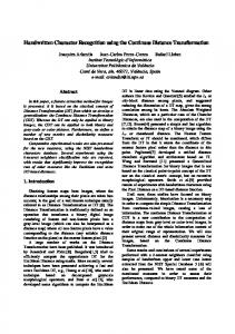
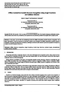
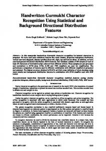
Figure 1:tion Illustration the computations and criterion forthat the denoising auto-encoder of x. Aof simple modification oftraining the auto-encoder Since training error tends to used to pre-train each layer of the deep architecture. Input x of the layer (i.e. raw input or • improves upon the classical auto-encoder and output of previous layer) s corrupted into x ˜ and encoded into code y by the encoder fθ (·).from right to left. Trajectori The decoder gθ0be (·) used mapstoy pretrain to reconstruction z, which is compared to the uncorrupted input xform of overfitting. Note that • can a deep network through the loss case, function LH (x, whose approximately In our KL(x||ˆ x) z), is used toexpected learn (b,value c, W )isand as done byminimized [6], we during • Pretrained networks start i training by tuning θ and θ0 . • For 2 and 3-layer networks

set Ci(x) = xi or 0, with a random subset (of a fixed size) selected for zeroing. "

" Here we chose to use the Denoising Auto-encoder [17] as the building block for these$ deep hierarchies of features, as it is simple to train and explain (see Figure 1, as well as tutorial and code there: http://deeplearning.net/tutorial), provides efficient inference, and yielded results comparable or better than RBMs in series of experiments [17]. During training, a Denoising Auto-encoder is presented with a stochastically corrupted version of the input and trained to reconstruct the uncorrupted input, forcing the hidden units to represent the leading regularities in the data. Here we use the random binary masking corruption (which sets to 0 a random subset of the inputs). Once it is trained, in a purely unsupervised way, its hidden units’ activations can be used as inputs for training a second one, etc. After this unsupervised pre-training stage, the parameters are used to initialize a deep MLP, which is fine-tuned by the same standard procedure used to train them (see previous section). The SDA hyper-parameters are the same as for the MLP, with the addition of the amount of corruption noise (we used the masking noise process, whereby a fixed proportion of the input values, randomly selected, are zeroed), and a separate learning rate for the unsupervised pre-training stage (selected from the same above set). The fraction of inputs corrupted was selected among {10%, 20%, 50%}. Another hyper-parameter is the number of hidden layers but it was fixed to 3 based on previous work with SDAs on MNIST [17]. The size of the hidden layers was kept constant across hidden layers, and the best results were obtained with the largest values that we could experiment with given our patience, with 1000 hidden units.

9

ing error, but a higher train

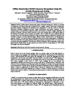
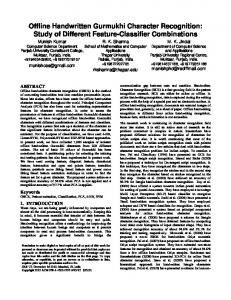
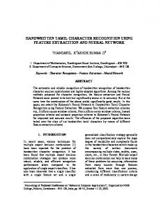
Figure 2: SDAx are the deep models. Error bars indicate a 95% confidence interval. 0 indicates that the model was trained on NIST, 1 on NISTP, and 2 on P07. Left: overall results of all models, on NIST and NISTP test sets. Right: error rates on NIST test digits only, along with the previous results from literature [19, 20, 21, 22] respectively based on ART, nearest neighbors, MLPs, and SVMs.

4

Experimental Results

The models are either trained on NIST (MLP0 and SDA0), NISTP (MLP1 and SDA1), or P07 (MLP2 and SDA2), and tested on either NIST, NISTP or P07, either on the 62-class task or on the 10-digits task. Training (including about half for unsupervised pre-training, for DAs) on the larger datasets takes around one day on a GPU-285. Figure 2 summarizes the results obtained, comparing humans, the three MLPs (MLP0, MLP1, MLP2) and the three SDAs (SDA0, SDA1, SDA2), along with the previous results on the digits NIST special database 19 test set from the literature, respectively based on ARTMAP neural networks [19], fast nearest-neighbor search [20], MLPs [21], and SVMs [22]. More detailed and complete numerical results (figures and tables, including standard errors on the error rates) can be found in Appendix. The deep learner not only outperformed the shallow ones and previously published performance (in a statistically and qualitatively significant way) but when trained with perturbed data reaches human performance on both the 62-class task and the 10-class (digits) task. 17% error (SDA1) or 18% error (humans) may seem large but a large majority of the errors from humans and from SDA1 are from out-of-context confusions (e.g. a vertical bar can be a “1”, an “l” or an “L”, and a “c” and a “C” are often indistinguishible). In addition, as shown in the left of Figure 3, the relative improvement in error rate brought by self-taught learning is greater for the SDA, and these differences with the MLP are statistically and qualitatively significant. The left side of the figure shows the improvement to the clean NIST test set error brought by the use of out-of-distribution examples (i.e. the perturbed examples examples from NISTP or P07). Relative percent change is measured by taking 100%× (original model’s error / perturbed-data model’s error - 1). The right side of Figure 3 shows the relative improvement brought by the use of a multi-task setting, in which the same model is trained for more classes than the target classes of interest (i.e. training with 10

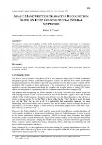
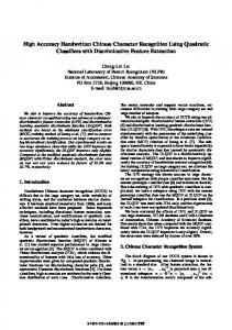
Figure 3: Relative improvement in error rate due to self-taught learning. Left: Improvement (or loss, when negative) induced by out-of-distribution examples (perturbed data). Right: Improvement (or loss, when negative) induced by multi-task learning (training on all classes and testing only on either digits, upper case, or lower-case). The deep learner (SDA) benefits more from both self-taught learning scenarios, compared to the shallow MLP. all 62 classes when the target classes are respectively the digits, lower-case, or upper-case characters). Again, whereas the gain from the multi-task setting is marginal or negative for the MLP, it is substantial for the SDA. Note that to simplify these multi-task experiments, only the original NIST dataset is used. For example, the MLP-digits bar shows the relative percent improvement in MLP error rate on the NIST digits test set is 100%× (single-task model’s error / multi-task model’s error - 1). The single-task model is trained with only 10 outputs (one per digit), seeing only digit examples, whereas the multi-task model is trained with 62 outputs, with all 62 character classes as examples. Hence the hidden units are shared across all tasks. For the multi-task model, the digit error rate is measured by comparing the correct digit class with the output class associated with the maximum conditional probability among only the digit classes outputs. The setting is similar for the other two target classes (lower case characters and upper case characters).

5

Conclusions and Discussion

We have found that the self-taught learning framework is more beneficial to a deep learner than to a traditional shallow and purely supervised learner. More precisely, the answers are positive for all the questions asked in the introduction. • Do the good results previously obtained with deep architectures on the MNIST digits generalize to a much larger and richer (but similar) dataset, the NIST special database 19, with 62 classes and around 800k examples? Yes, the SDA systematically outperformed the MLP and all the previously published results on this dataset (the ones that we are aware of), in fact reaching human-level performance at around 17% error on the 62class task and 1.4% on the digits, and beating previously published results on the same data. • To what extent do self-taught learning scenarios help deep learners, and do they help them more than shallow supervised ones? We found that distorted training examples 11

not only made the resulting classifier better on similarly perturbed images but also on the original clean examples, and more importantly and more novel, that deep architectures benefit more from such out-of-distribution examples. MLPs were helped by perturbed training examples when tested on perturbed input images (65% relative improvement on NISTP) but only marginally helped (5% relative improvement on all classes) or even hurt (10% relative loss on digits) with respect to clean examples . On the other hand, the deep SDAs were significantly boosted by these out-of-distribution examples. Similarly, whereas the improvement due to the multi-task setting was marginal or negative for the MLP (from +5.6% to -3.6% relative change), it was quite significant for the SDA (from +13% to +27% relative change), which may be explained by the arguments below. In the original self-taught learning framework [4], the out-of-sample examples were used as a source of unsupervised data, and experiments showed its positive effects in a limited labeled data scenario. However, many of the results by Raina et al. [4] (who used a shallow, sparse coding approach) suggest that the relative gain of self-taught learning vs ordinary supervised learning diminishes as the number of labeled examples increases. We note instead that, for deep architectures, our experiments show that such a positive effect is accomplished even in a scenario with a large number of labeled examples, i.e., here, the relative gain of self-taught learning is probably preserved in the asymptotic regime. Why would deep learners benefit more from the self-taught learning framework? The key idea is that the lower layers of the predictor compute a hierarchy of features that can be shared across tasks or across variants of the input distribution. A theoretical analysis of generalization improvements due to sharing of intermediate features across tasks already points towards that explanation [24]. Intermediate features that can be used in different contexts can be estimated in a way that allows to share statistical strength. Features extracted through many levels are more likely to be more abstract (as the experiments in Goodfellow et al. [3] suggest), increasing the likelihood that they would be useful for a larger array of tasks and input conditions. Therefore, we hypothesize that both depth and unsupervised pre-training play a part in explaining the advantages observed here, and future experiments could attempt at teasing apart these factors. And why would deep learners benefit from the self-taught learning scenarios even when the number of labeled examples is very large? We hypothesize that this is related to the hypotheses studied in Erhan et al. [23]. Whereas in Erhan et al. [23] it was found that online learning on a huge dataset did not make the advantage of the deep learning bias vanish, a similar phenomenon may be happening here. We hypothesize that unsupervised pre-training of a deep hierarchy with self-taught learning initializes the model in the basin of attraction of supervised gradient descent that corresponds to better generalization. Furthermore, such good basins of attraction are not discovered by pure supervised learning (with or without self-taught settings), and more labeled examples does not allow the model to go from the poorer basins of attraction discovered by the purely supervised shallow models to the kind of better basins associated with deep learning and self-taught learning. A Flash demo of the recognizer (where both the MLP and the SDA can be compared) can be executed on-line at http://deep.host22.com.

12

Appendix I: Detailed Numerical Results These tables correspond to Figures 2 and 3 and contain the raw error rates for each model and dataset considered. They also contain additional data such as test errors on P07 and standard errors. Table 1: Overall comparison of error rates (± std.err.) on 62 character classes (10 digits + 26 lower + 26 upper), except for last columns – digits only, between deep architecture with pre-training (SDA=Stacked Denoising Autoencoder) and ordinary shallow architecture (MLP=Multi-Layer Perceptron). The models shown are all trained using perturbed data (NISTP or P07) and using a validation set to select hyper-parameters and other training choices. {SDA,MLP}0 are trained on NIST, {SDA,MLP}1 are trained on NISTP, and {SDA,MLP}2 are trained on P07. The human error rate on digits is a lower bound because it does not count digits that were recognized as letters. For comparison, the results found in the literature on NIST digits classification using the same test set are included. Humans SDA0 SDA1 SDA2 MLP0 MLP1 MLP2 [19] [20] [25] [22]

NIST test 18.2% ±.1% 23.7% ±.14% 17.1% ±.13% 18.7% ±.13% 24.2% ±.15% 23.0% ±.15% 24.3% ±.15%

NISTP test 39.4%±.1% 65.2%±.34% 29.7%±.3% 33.6%±.3% 68.8%±.33% 41.8%±.35% 46.0%±.35%

13

P07 test 46.9%±.1% 97.45%±.06% 29.7%±.3% 39.9%±.17% 78.70%±.14% 90.4%±.1% 54.7%±.17%

NIST test digits 1.4% 2.7% ±.14% 1.4% ±.1% 1.7% ±.1% 3.45% ±.15% 3.85% ±.16% 4.85% ±.18% 4.95% ±.18% 3.71% ±.16% 2.4% ±.13% 2.1% ±.12%

Table 2: Relative change in error rates due to the use of perturbed training data, either using NISTP, for the MLP1/SDA1 models, or using P07, for the MLP2/SDA2 models. A positive value indicates that training on the perturbed data helped for the given test set (the first 3 columns on the 62-class tasks and the last one is on the clean 10-class digits). Clearly, the deep learning models did benefit more from perturbed training data, even when testing on clean data, whereas the MLP trained on perturbed data performed worse on the clean digits and about the same on the clean characters. SDA0/SDA1-1 SDA0/SDA2-1 MLP0/MLP1-1 MLP0/MLP2-1

NIST test 38% 27% 5.2% -0.4%

NISTP test 84% 94% 65% 49%

P07 test 228% 144% -13% 44%

NIST test digits 93% 59% -10% -29%

Table 3: Test error rates and relative change in error rates due to the use of a multi-task setting, i.e., training on each task in isolation vs training for all three tasks together, for MLPs vs SDAs. The SDA benefits much more from the multi-task setting. All experiments on only on the unperturbed NIST data, using validation error for model selection. Relative improvement is 1 - single-task error / multi-task error.

MLP-digits MLP-lower MLP-upper SDA-digits SDA-lower SDA-upper

single-task setting 3.77% 17.4% 7.84% 2.6% 12.3% 5.93%

multi-task setting 3.99% 16.8% 7.54% 3.56% 14.4% 6.78%

14

relative improvement 5.6% -4.1% -3.6% 27% 15% 13%

References [1] Yoshua Bengio. Learning deep architectures for AI. Foundations and Trends in Machine Learning, 2(1):1–127, 2009. Also published as a book. Now Publishers, 2009. [2] Honglak Lee, Chaitanya Ekanadham, and Andrew Ng. Sparse deep belief net model for visual area V2. In NIPS’07, pages 873–880. MIT Press, Cambridge, MA, 2008. [3] Ian Goodfellow, Quoc Le, Andrew Saxe, and Andrew Ng. Measuring invariances in deep networks. In NIPS’09, pages 646–654. 2009. [4] Rajat Raina, Alexis Battle, Honglak Lee, Benjamin Packer, and Andrew Y. Ng. Selftaught learning: transfer learning from unlabeled data. In ICML 2007, pages 759–766, 2007. [5] J. Weston, F. Ratle, and R. Collobert. Deep learning via semi-supervised embedding. In ICML 2008, 2008. [6] Ronan Collobert and Jason Weston. A unified architecture for natural language processing: Deep neural networks with multitask learning. In ICML 2008, pages 160–167, 2008. [7] P. Vincent, H. Larochelle, Y. Bengio, and P.-A. Manzagol. Extracting and composing robust features with denoising autoencoders. In ICML 2008, 2008. [8] R. M. Haralick, S. R. Sternberg, and X. Zhuang. Image analysis using mathematical morphology. IEEE Trans. Pattern. Anal. Mach. Intel., 9(4):532–550, 1987. [9] J. Serra. Image Analysis and Mathematical Morphology. Academic Press, 1982. [10] Patrice Simard, David Steinkraus, and John C. Platt. Best practices for convolutional neural networks applied to visual document analysis. In ICDAR, pages 958–962, 2003. [11] Hugo Larochelle, Yoshua Bengio, Jerome Louradour, and Pascal Lamblin. Exploring strategies for training deep neural networks. Journal of Machine Learning Research, 10: 1–40, 2009. [12] Goeffrey E. Hinton, Simon Osindero, and Yee Whye Teh. A fast learning algorithm for deep belief nets. Neural Computation, 18:1527–1554, 2006. [13] M. Ranzato, C. Poultney, S. Chopra, and Y. LeCun. Efficient learning of sparse representations with an energy-based model. In NIPS’06, 2007. [14] Yoshua Bengio, Pascal Lamblin, Dan Popovici, and Hugo Larochelle. Greedy layer-wise training of deep networks. In NIPS 19, pages 153–160. MIT Press, 2007. [15] Ruslan Salakhutdinov and Geoffrey E. Hinton. Deep Boltzmann machines. In AISTATS’2009, volume 5, pages 448–455, 2009. [16] Hugo Larochelle, Yoshua Bengio, Jerome Louradour, and Pascal Lamblin. Exploring strategies for training deep neural networks. JMLR, 10:1–40, 2009. 15

[17] Pascal Vincent, Hugo Larochelle, Yoshua Bengio, and Pierre-Antoine Manzagol. Extracting and composing robust features with denoising autoencoders. In ICML’08, pages 1096–1103. ACM, 2008. [18] P.J. Grother. Handprinted forms and character database, NIST special database 19. In National Institute of Standards and Technology (NIST) Intelligent Systems Division (NISTIR), 1995. [19] Eric Granger, Robert Sabourin, Luiz S. Oliveira, and Catolica Parana. Supervised learning of fuzzy artmap neural networks through particle swarm optimization. JPRR, 2(1): 27–60, 2007. [20] Juan Carlos P´erez-Cortes, Rafael Llobet, and Joaquim Arlandis. Fast and accurate handwritten character recognition using approximate nearest neighbours search on large databases. In IAPR, pages 767–776, London, UK, 2000. Springer-Verlag. ISBN 3-54067946-4. [21] L.S. Oliveira, R. Sabourin, F. Bortolozzi, and C.Y. Suen. Automatic recognition of handwritten numerical strings: a recognition and verification strategy. IEEE Trans. Pattern Analysis and Mach. Intelli., 24(11):1438–1454, 2002. [22] J. Milgram, M. Cheriet, and R. Sabourin. Estimating accurate multi-class probabilities with support vector machines. In Int. Joint Conf. on Neural Networks, pages 906–1911, 2005. [23] Dumitru Erhan, Yoshua Bengio, Aaron Courville, Pierre-Antoine Manzagol, Pascal Vincent, and Samy Bengio. Why does unsupervised pre-training help deep learning? Journal of Machine Learning Research, 11:625–660, 2010. [24] Jonathan Baxter. Learning internal representations. In Proceedings of the 8th International Conference on Computational Learning Theory (COLT’95), pages 311–320, Santa Cruz, California, 1995. ACM Press. URL http://citeseer.ist.psu. edu/baxter95learning.html. [25] L.S. Oliveira, R. Sabourin, F. Bortolozzi, and C.Y. Suen. Automatic recognition of handwritten numerical strings: a recognition and verification strategy. IEEE Trans. Pattern Analysis and Mach. Intelli., 24(11):1438–1454, November 2002. ISSN 0162-8828. doi: 10.1109/TPAMI.2002.1046154.

16