Abstract- The purpose of this paper is to present a method- ology for the evaluation of the Defect Level in an IC design environment. The methodology is based ...
1286
IEEE TRANSACTIONS ON COMPUTER-AIDED DESIGN OF INTEGRATED CIRCUITS AND SYSTEMS, VOL. 15, NO. 10, OCTOBER 1996
JosC Teixeira de Sousa, Fernando M. Gonqalves, J. Paul0 Teixeira, Cristoforo Marzocca, Francesco Corsi, Associate, IEEE, and T. W. Williams, Fellow, IEEE
Abstract- The purpose of this paper is to present a methodology for the evaluation of the Defect Level in an IC design environment. The methodology is based on the extension of Williams-Brown formula to nonequiprobable faults, which are collected from the IC layout, using the information on a typical IC process line defect statistics. The concept of weighted fault coverage is introduced, and the Defect Level (DL) evaluated for the Poisson and the negative binomial yield models. It is shown that DL depends on the critical areas associated with undetected faults, and their correspondentdefect densities. Simulationresults are presented, which highlight that the classic single Line StuckAt (LSA) fault coverage is a unreliable metric of test quality. Moreover, results show that the efficiency of a given set of test patterns strongly depends on the physical design and defect statistics.
NOMENCLATURE BRI DL FL LOP LSA PhFM TSOP
bridging fault defect level fault level, DL evaluated by LSA fault coverage line open fault gate level line stuck-at fault physical failure mode transistor stuck-open fault
I. INTRODUCTION N order to achieve the high standards of electronic products quality, it is mandatory to evaluate test quality. The zero defects strategy leads, in practice, to the definition of Defect Levels (DL) (or escape rates) as low as 100 ppm (parts per million) or less. We refer to Defect Level [1] and [2] as the percentage of defective chips that successfully pass the production test and, thus, are marketed as good. Hence, at the production stage, DL should be viewed an important indicator of test quality. Test preparation is carried out in the design phase of the product development. However, test quality, in the digital IC design environment, is usually assessed by the fault coverage. Manuscript received May 19, 1994; revised March 7, 1995 and May 24, 1996. This work was supported in part by the EEC, in the context of Esprit 7107 Project, ARCHIMEDES; also, supported by the JNICT (Portugal) and the “Minister0 dell’Universit8 della Ricerca Scientifica e Tecnologica” (MURST, Italy). This paper was recommended by Associate Editor W. Maly. J. Teixeira de Sousa, F. M. Gonqalves, and J. P. Teixeira are with INESC, IST, Technical University of Lisbon, Lisbon, Portugal. C. Marzocca and F. Corsi are with Politecnico di Bari, Bari, Italy. T. W. Williams is with IBM Corporation, Boulder, CO 80301 USA. Publisher Item Identifier S 0278-0070(96)07468-4.
In industry, the fault coverage is estimated as the percentage of single Line Stuck-at (LSA) faults which are detectable by a set of test patterns, and is evaluated by gate-level fault simulation (this could also be expanded to model other types of faults, such as delay faults). The Defect Level (DL) may be estimated using Williams-Brown equation [ 11, relating DL with the yield Y and the fault coverage T as
D L = 1 - Y(l-T).
(1)
This equation was derived under the assumption of equiprobable faults, and it can be used by the chip manufacturer to estimate DL after a production test of defined coverage. However, the IC designer has not sufficient data to predict DL, and thus to evaluate the test quality. Moreover, it has been proved, especially for CMOS designs, that single LSA fault coverage is not synonymous with defect coverage [3]-[6]. In fact, physical defects, induced or enhanced during IC manufacturing, are the real cause of circuit faults; those which modify the dc connectivity of adjacent conducting or semiconducting regions [7] (or the device characteristics) are referred as critical defects. Under this perspective, test quality should evaluate the ability of the test patterns to cover critical defects. Unfortunately, the common practice is that the fault list is compiled on the basis of a purely topological description of the circuit (usually, gate level), without any reference to its layout, or its physical structure. Hence, some faults which actually affect the circuit are disregarded, whereas other faults which cannot physically occur are included in the fault list. In view of such abstract fault model, equiprobable faults are assumed, which strongly deviates from the reality. As a consequence, single LSA fault coverage, T , can be a misleading metric for test quality [4], [ 5 ] , [8]-[ll], and both Y and T may loose validity and meaning, as confirmed also by observation on production chips [ 121. The purpose of this paper is to present a methodology for the evaluation of the Defect Level in an IC design environment. The methodology is based on the extension of the Williams-Brown equation [ 11 to nonequiprobable faults [ 131 and [14], which are collected from the IC layout, by exploiting the concept of critical area, and using the information on a typical IC process line defect statistics (see, e.g., [15]). Section I1 introduces the extension of (l), the concept of a weighting factor, associated with the probability of occurrence of each fault, and the definition of a weighted fault coverage 0. The evaluation of the faults probabilities, for different
0278-0070/96$05,00 0 1996 IEEE
TEIXEIRA DE SOUSA ef al.: DEFECT LEVEL EVALUATION
1287
yield models, is presented in Section 111, in which a physical The last equation clearly shows that the Defect Level only significance to R is given. Section IV reviews the software depends on the probability of occurrence of the undetected package used to extract the realistic fault list and to compute faults. In other words, (1-DL) is the partial yield associated Y , R, and DL and presents some illustrative simulation with the undetected faults. Given the identity x = eln (z), or, in examples. A final discussion is included in Section V. general, ic = a l o R a (%) where ic > 0, (7) can also be written as 11. DEFECTLEVELFOR NONEQUIPROBABLE FAULTS
Let us define the event A as the real fault-free case, i.e., the case in which none of the n faults, assumed possible to occur (and thus included in the fault set) is present on the chip. Moreover, let B represent the event which refers to successful testing for m out of the n assumed faults (rn 5 n). Assuming equiprobable faults, with p as the probability of a fault occurring, P ( A ) =: (1 - p)" is the probability of a good chip and, by definition, is equal to the yield (referred to the chosen fault model). P(L3) = (1 - p)" is the probability of having a chip not affected by rn out of n faults. P(A1B) is the probability of having a good chip after a test whose fault coverage is T = m/n,. This, by definition, coincides with 1-DL. By application of Bayes rule [16]
= 1 - DL.
(1 1)
Consequently, we may define a new parameter, the weighted fault coverage R as and, since P(B1A) = 1,
n m
In
0=
(1 - P j )
j=1
(12)
and conclude that
As a consequence,
which is the well-known formula presently employed for equiprobable faults. Assuming now that nonequiprobable independent faults may occur, denoting p j the probability of occurrence of fault j , and reordering the fault list in such a way that the first m are the ni out of n detected faults, we have
P ( A ) =Y
i.e., we can retain (1) for nonequiprobable faults, if the concept of weighted fault coverage is introduced, rather than the one associated with the equal probability assumption. R is still a fault coverage, as it compares detected faults with the entire fault set; however, it takes into account the probabilities of nonoccurrence (1 - p j ) of detected faults, as compared to the probabilities of nonoccurrence of all likely faults. Of course, for equiprobable faults, R reduces to T . At this stage, and for reasons that will become apparent in the following, a weighting factor of a fault w j is introduced as [13]
n
wj = j=1
-In (1 - p j ) .
The above equations can thus be written as
m
=r-(l-Pi)
Y = exp
i=l n
m
(1 - Pi)
(
-
R j=1 n
(1-Pi)
=
D L = 1 - exp
i=m+l
1 - DL.
(7)
(14)
1288
IEEE TRANSACTIONS ON COMPUTER-AIDED DESIGN OF INTEGRATED CIRCUITS AND SYSTEMS, VOL. 15, NO. 10, OCTOBER 1996
These equations are general, since Y , 0,and DL are dependent on the fault probabilities of occurrence, which can be computed for different yield models. As it will be seen in Section 111-A, for the Poisson yield model, a physical significance can be attributed to w3 and 0. For a given defects statistics and physical design, it is expected that a wide spread of fault probabilities will occur in the fault set. This will likely have an impact on 0, and thus on DL. Moreover, it may be rewarding to partition the fault set in subsets, according to the different Physical Failure Modes (PhFM's), and/or to different topological attributes, that can help discriminating hard from easy to detect faults [lo]. Hence, for each subset (or fault class), we introduce the concept of Class Fault Incidence, F I,, as
3=1
FIk =
~
2
where K is the random variable "number of faults" and 6' is the probability that a randomly selected defect will result in a fault. The probability of a given elementary electrical fault is the probability of having at least one defect landing in the critical area defined for that fault:
P(fauZt) = P ( K = 1IR = 1 ) P ( R= 1) + [ P ( K= 1IR = 2) + P ( K = 21R = a)] ' P(R= 2) + " . c a r
WL
and a correspondent class fault coverage,
2
(22)
or
2=1
0 k=
probability that k out of r of these defects will result in faults (i.e., defect landing in the critical area):
r=l k=l 0 k ,
as
WI)
3=1 ~
F W , 2=1
where m k are the detected faults of class k . After some manipulation, the weighted, global fault coverage R can be written as c
R=
FIkS2k
(20)
k l
r=l
= 1 - exp ( - R )
where c is the total number of fault classes. 111. EVALUATING INDIVIDUAL FAULTPROBABILITIES
In order to compute Y , R,and DL, we need to evaluate the probabilities of occurrence of the faults p , in the fault set. We assume that a circuit fault is a consequence of a critical defect present on the chip. The physical defects under consideration are spot defects, which can be related in some way to the lithographic masks of the process [7] and [17].
Now, in the joint probability expression, P ( f auZt, d e f e c t ) = P(fauZtldefect)P(defect),we may evaluate the conditional probability from (22) for k = 1 and r = 1, yielding
P(fnuZt1defect) = P ( K = 1 / R= I )
=e where A, is the critical area [18], given by
A. Uniform Distribution of Defects (Poisson Yield Model)
Assume a spot defect of a given diameter P . In general, the number of spot defects landing on a chip is a random variable R for which a Poisson distribution function is hypotized. Therefore, the probability of having exactly r defects is given by
P(R= r) =
exp (-R)X r!
where 75: = A D is the product of the chip area, A, times the average number of defects per unit area, D (defect density). Assuming the defects are independent of each other, a Bernoulli trials model can be applied to calculate the
and f~ (Q) is the defect size distribution function. Hence, 6' has a simple geometrical interpretation: it is the ratio A,/A in the hypothesis of uniformly distributed defects. By substituting in (27), we finally obtain
P(fauZt) = 1 - exp (-A,D)
(30)
which shows that to evaluate the probability of a given fault, it is required to know the average defect density and the critical area for that fault.
TElXElRA DE SOUSA et al.: DEFECT I,EVEL EVALUATION
1289
Clearly, a fault may result from the union of a set of disjoint events. For instance, a short between two electrical nodes may result from shorts between different wires, of different layers (such as shorts between two metal-1 lines, and between two poly lines). In this case, the effective critical area is the sum of the elementary critical areas, each weighted by its defect density, corresponding to the elementary faults [7]. We refer to elementary faults as those associated with a single circuit topology (e.g., short between nodes 51 and Q), and a single PhFM; examples of PhFM’s are shorts between poly lines, or open Alldiffusion contacts. On the contrary, we may wish to analyze separately each elementary fault, to assume for each PhFM a defect density, D,, and then to define for each of these faults a critical area, A , . At present, there are several tools available for critical areas evaluation [9] and [ 191-[24]. In the software package described in (section IV [9]), such approach is followed. Under the Poisson yield model, and assuming elementary faults, we can thus write for the weighting factor of fault j WJ
=-lm(1 - p 3 ) = A, .D,
(31)
and, hence,
Y = exp m,
I
P9-I statistics
Testability report; Y
c
.
FLOC
FANCY I
I
I
c
Test patterns
SWIFT
f
O.DL ~~
,
I
Fig. 1. Software package for defect level evaluation.
The important point from all these equations is that, if all the defect densities were to increase by a factor ,8, the yield will decrease (32), R, being a ratio, will remain the same (33), and DL will increase, as expected. This work establishes a mathematical basis in order to quantify a good layout for a given set of defect densities.
B. Defect Clustering (Negative Binomial Keld Model) The generalized negative binomial model is commonly employed to account for defect clustering [25] and is characterized by b
( -2 ) A,D,
-
-. Technology
where aj is the clustering parameter. The smaller the a; value, the stronger the clustering. In this case, although the faults are no longer independent, the general yield expression (S), still holds [25]. As a consequence, we may still use the general equation (12) and (13). Under the assumption of this yield model, the weighting factor has a more complex dependence on the critical areas and defect densities, since
AiDi i=l
w; = - l n ( 1 - p j ) FIk=
.
j=l 7L
ADZ
(35)
=a3 In
Aj Dj
(37)
i=l
However, (15)-( 17) still apply, provided that (37) is used As a consequence, for this yield model, a physical significance for the evaluation of wj.As a general conclusion, we may can be attributed to wj,0, and FIk: point out that the influence of the yield model on DL can wj-represents the average number of critical defects be computed from (15)-(17), where the weighting factors are associated with fault j ; evaluated in accordance to the specific yield model, which R-describes the percentage of tested critical area (i.e., may include clustering. associated with detected faults), weighted by the relative defects densities. In fact, due to (33), where ratios of IV. SIMULATION EXAMPLES AjDj occur, only the relative defect density of each individual PhFM influences the weighted fault coverage. Of course, if only one PhFM is considered as likely, R A. Sojiware System In order to evaluate, in the IC design environment, the represents simply the ratio of two critical areas, the tested area, divided by the total critical area. In our work, we Defect Level, and to estimate the influence of the defect take the defect density of shorts between metal-l lines, statistics and layout style, the software package depicted in Fig. 1 has been used. Do, as reference. Here, L I F T is the circuit and realistic fault extractor. FIk-represents the percentage of critical area associated with fault class k , weighted by the relative densities of Together with the circuit netlist (at transistor level), L I F T outputs a realistic fault list. Each fault has assigned to it a set the defects causing the faults.
IEEE TRANSACTIONS ON COMPUTER-AIDED DESIGN OF INTEGRATED CIRCUlTS AND SYSTEMS, VOL. 15, NO. 10, OCTOBER 1996
1290
TABLE I LIKELYPHYSICAL FAILURE MODES(PHFM) IN A DIGITALCMOS PROCESS Layer(s) Diffusion Polysilicon Metal-1
ad
short
a,
75 FI(%) 50
open short open short
aP
25
Failure Nature open
Relative Density
100
100
FI(%? SO
25
DP %Ill
I
1.0
0
25
Metal2
50
75
100
0
?#FAULTS (Yo) short
ml/poly contacts vias
of attributes, namely, the fault type, the PhFM originating it, and the weighting factor, w j , evaluated as described above. At present, in L I F T , two basic types of faults are defined, BRI (bridging) and LOP (Line Open) faults. PhFM’s are user’s defined, being usually, for a digital CMOS process, interconnection failures and device failures, as described in Table I. In this table, MOS transistor drain to source shorts are taken into account, as poly opens occurring in channel areas. Other failures can be considered, as, for instance, gate oxide shorts (due to thin oxide pinholes), or metal-1 opens due to metal-l/poly step coverage problems. However, as no defect statistics for these failure mechanisms are available to the authors, these failure modes were not included. Fault collapsing is performed by C L I F T . Basically, topologically equivalent faults associated with the same conductive layer (e.g., shorts in parallel, opens in series) are collapsed. Therefore, topologicaily equivalent faults caused by different PhFM’s are not collapsed, in order to allow the identification of the elementary faults. An additional advantage of defining 7uj as in (14) is the easiness of computing the weighting factor of the remaining faults. In fact, when eliminating faults from the fault set, without distorting the representativeness of the faults, the weighting factor of each remaining fault (representative of itself and of the collapsed faults) is evaluated by simply adding the w j of the remaining fault to the U J of ~ the collapsed faults; for the Poisson yield model, this corresponds to adding the critical areas of the equivalent faults. Fault classification is carried out by FANCY, using a refined classification of BRI and LOP faults proposed in [lo], to discriminate hard from easy to detect fault subsets. FANCY also computes FIk and Y , and estimates R and DL. FANCY further discriminates TSOP (Transistor Stuck-Open) faults, since this type of faults has received considerable attention in the literature, in the last decade. TSOP faults are a subtype of LOP faults which disconnect single channel terminals (source or drain) from the broken nodes. Switch-level fault simulation can be performed using SWIFT, which computes RI,and R, and finally DL. Such computation can highlight the contribution of the different fault classes to the overall Defect Level value. For layout and fault inspection, an additional tool, FLOC, is available. FLOC is a graphics display program, which allows the visualization of the layout and the faults location and attributes, as well as bar or pye charts of the fault incidences, according to different fault classes or PhFM’s.
50
25
75
100
#FAULTS (%) (b)
(a) 100
F I j %50 Y
~
25
0
25
50
75
#FAULTS (%) (C)
103
0
50
25
75
100
#FAULTS (%)
(4
Fig. 2. Fault incidences versus the percentage of faults, for different physical designs c432a, b and defect statistics. (a) c432dR1. (b) c 4 3 2 m 2 . (c) c432biR1. (d) c432biR2.
B. Simulation Results The results reported in this paper deal with: two CMOS physical designs of the same logic network (i.e., the c43 2 , an ISCAS benchmark circuit [22]), obtained with two different cell libraries and the same place&route software system. These two physical designs, referred as c 4 3 2 a and b, show the influence of the cell library on R and DL; two defect statistics, one from an European IC manufacturer’s data (dominated by bridging defects, and referred as Rl), and a more balanced defects statistics (R2) (balanced in terms of opens and shorts), to show how defects statistics modulates wj, FIh, Y , R, and DL. In R 2 , equal relative defect densities are assumed. Both statistics include the full spectrum of likely PhFM’s depicted in Table I. Numerical results have been computed for the Poisson yield model. two defect densities of metal-1, namely Do = 2 and 0.8 defects/cm2 (and the same relative defect densities (relative to metal-1 density) for the different PhFM’s), to highlight the effect on Y but not on R. Comparison, of course, is also made with the equiprobable approach (T = m / n ) ,and with the DL values, computed from the realistic Y values, and gate-level, single line stuck-at fault coverages (referred as FL, or fault level). Fig. 2 shows the influence of the defects statistics on the nonequiprobability of the extracted faults. The 45” line corresponds to the equiprobable case. It can be seen that the real process line defects statistics ( R l ) leads to less than 50% of the extracted BRI faults accounting for more than 90% of the fault incidence. This fact must be taken into account when test preparation costs, namely test generation and fault simulation costs, are being defined. Furthermore, if BRI faults
TEIXEIRA DE SOUSA et al.: DEFECT L.EVEL EVALUATION
1291
TABLE I1
1.Oe-04
metall
-i
1.k-05
# Fault weight
FAULTCOVERAGE, WEIGHTED FAULT COVERAGE, YIELD,DEFECT, AND FAULT LEVEL Example c432a/R1/2 c432a/R2/2 -.-2b/R1/2 c432b/R2/2 c432b/R1/.8
1.0"
i.oe-n7
200
400
Number o f BRI faults
I
I
I
T (%) 91.4 91.4 , 91.4 I 91.4 I 91.4 1
Q (%)
I Y (%) I DL (ppm) I FL (ppm)
98.6 I 791.1 97.7 76.6 97.5 I
99.91 I 99.61 99.88 99.54 99.95 1
12.5 813.6 26.7 1089.7 11.5
I
1
77.4 356.0 103.3 396.4 43.0
600
Fig. 3 . Weighting factors of ranked metal-2, metal-1 and poly shorts associated with c432a/~1and Do = 2 defects/cm2.
are very likely to occur (as in this example), one should include them in the fault model as target faults, to obtain low Defect Levels. In the past, a number of papers and considerable energy has been directed at research to develop automatic test pattern generation tools for TSOP faults. Also, a large effort was undertaken to find such physical examples, with limited results. The work reported in this paper shows that, in fact, the TSOP faults give a negligible contribution to R (due to very low fault incidences), even for processes where open faults are significant (R2), and provides a physical explanation for it. For such processes, effort should be directed at more general LOP faults (splitting the branches converging to the broken node in unique subsets, physically possible), not at TSOP faults. In order to further highlight the influence of the fault's nonequiprobability, Fig. 3 depicts the fault weights (closely related to their probability of occurrence) of metal-2, metal-l and poly shorts, in one of the examples. It can be seen that a significant number of extracted faults are associated with limited critical areas and/or defect densities, and thus only weakly influence the weighted fault coverage. Also, shorts between long interconnection lines (especially, metal lines) dominate this standard cell layout. Hence, routing can play an important role in the Defect Level of digital IC's. Finally, in Table 11, a comparison is made among the different physical designs, defect statistics and defect densities. The deterministic set of test patterns used was a stuck-at test set, i.e., it was derived for Line Stuck-At (LSA) fault detection, leading to T := 91.4%. The corresponding weighted fault coverage is significantly different from T . In fact, for R1, dominated by BFU faults, fl is consistently higher than T . On the contrary, assuming a more balanced defects statistics (R2), lower values of R are obtained. For more practical and large circuits, we observe that, in general, when T = 1is approached by the LSA test set, R is still well below 100%. From this we can conclude that, in general, significantly different values of T and f2 occur. Hence, it can be seen from Table 11: that it is very difficult, for the circuit designer, to accurately evaluate DL using only the classical approach, where T and an estimated yield are used. Here, we used for Y the computed values from the realistic fault list, and, as a consequence, the estimated value (FL) can vary from 43-396 ppm. This variability is caused by different values of Y . The high values obtained for Y in this
example are due to the small layout area (less than 1 mm2). The classical fault coverage T is thus a unreliable metric for test quality. Moving to the weighted fault coverage, it can be seen that open faults are more difficult to detect by this test pattern, as R is around 98% for R1, but only around 78% for R2. Such a difference produces a very significant change on DL; for instance, for the c432a circuit, for R1,DL = 12.5 ppm, while for R2,DL = 813.6 ppm. These results put into evidence that the product Defect Level strongly depends on the defect statistics. Another important conclusion is that the physical design can significantly decrease DL. In fact, for the R1 and Do= 2 defectskm' on the metal-1 lines, DL can vary from 26.7 down to 12.5 pprn (almost half the value) moving from the c432b to the c4 32a physical implementation. This improvement not only enhances the test efficiency (measured by the 92 increase) but also enhances the design, increasing product quality. Finally, by improving the process control, and thus reducing the defect density (as shown, by moving from Do = 2 to 0.8 defects/cm2 on the metal-1 lines), an almost linear dependence of DL on Do (due to the high values of Y and 0) can be observed.
V. CONCLUSIONS In conclusion, a methodology for the evaluation of the Defect Level in an IC design environment has been proposed. The methodology uses an automatic translation from physical defects to circuit faults on the basis of experimental information from the process line. This is a rather different approach as compared to the original Inductive Fault Analysis (IFA) approach [17], leading to a computationally much more affordable solution, as it can be seen from the estimates of the number of Monte Carlo trials reported in [7]. The methodology is based on an extension of the Williams-Brown model for the Defect Level to nonequiprobable faults. The probability of occurrence of each individual fault is evaluated, provided that a critical area can be defined for it, either without or with defect clustering (Poisson and negative binomial yield models). A weighting factor w3 has been introduced, which, for the normal distribution, describes the average number of critical defects associated with fault j. The concepts of weighted fault incidences (FIk) and coverage (0)were also introduced, providing quantitative measures of the relative importance of nonequiprobable faults, and of the efficiency of a given set of test patterns to cover the likely faults, respectively. R assumes the meaning of a more general fault coverage figure.
1292
IEEE TRANSACTIONS ON COMPUTER-AIDED DESlGN OF INTEGRATED ClRCUITS AND SYSTEMS, VOL.
implies the minimization of the untested critical area, the Part Of it associated with large defect density failure mechanisms. For a given - defects statistics, the -general goal is, while maximizing the yield, to minimize the critical areas of hard to detect faults. In fact, the total critical area, modulated by the different defect densities, determines the product yield. The large spread in p j of the different faults is not, in itself, a reliable indication On their hp0rtanCe to test quality. In fact, large p j lead to large fault incidences. However, it does not provide information on the easiness of detection: low incidence fault classes can be hard to test (low Rk), while high incidence classes may be easy to test. Equation (20) provides the way to quantify the relative contribution of each class to R and thus to DL. The problem is that an identification of the untested critical area (or of the hard to detect faults) is not known prior to physical design, and fault simulation. The proposed fault classification [lo], based on topological attributes, represents a first step in this direction. Furthermore, it was demonstrated, for a digital CMOS process, that the fault’s nonequiprobability strongly modulates the fault list, R and DL. Bridging faults have been found as dominant faults, for which the stuck-at test sets are relatively efficient in covering these nontarget faults. Transistor stuckopen faults exhibit a negligible influence, which points out that researchers may have overemphasized their importance. However, LOP faults are difficult to be detected by stuck-at test sets. When the classical LSA fault model was considered, is was verified that it constitutes a unreliable metric for DL evaluation, and thus for test quality evaluation. Additionally, it was shown in this paper that DL depends on the layout style, namely on the cell library and the routing pattern; this leads us to the conclusion that layout level design for testability may be rewarding, especially to achieve extremely low values of DL, provided it may be automatable. Moreover, DL strongly depends on the defect statistics (defect size, distribution, and densities); hence, layout sensitivity to different PhFM’s should be analyzed, to improve IC quality. The proposed methodology provides a mathematical basis to carry out such analysis. Finally, one may argue on the usefulness of the approach presented in this work, when dealing with large digital IC’s. Nevertheless, the methodology is applicable to different circuit sizes, provided that data handling, namely the fault list, is manageable. For a standard cell layout style, preprocessed extraction of the cells faults can be carried out. After cell placement and routing, routing faults can be extracted, for each block, and the complete fault set can thus be built. If two large fault sets result, statistical fault sampling can further be performed. REFERENCES [1] T. W. Williams and N. C. Brown, “Defect level as a function of fault coverage,” IEEE Trans. Comput., vol. C-30, pp. 987-988, Dec. 1981. 121 V. D. Agrawal, S. C. Seth, and P. Agrawal, “Fault coverage requirements in production testing of LSI circuits,” IEEE J. Solid-State Circuits vol. sc-17, pp. 57-61,1982. [3] R. L. Wadsack, “Fault modeling and logic simulation of CMOS and NMOS integrated circuits,” Bell Syst. Tech. J., vol. 57, no. 2, pp. 1449-74, May/June 1978.
[5] 161 [7]
[SI
[9] [IO]
1111 1121 [13]
[14] 1151 1161 [17] [18] [19] [20] 1211 1221 [23] 1241
~~
[25] [26]
15,
NO.
10,
OCTOBER 1996
models, physical defect coverage, and I D D Qtesting,” in Proc. Custom Integ. Circuits ConJ: (CICC), 1991, pp. 13.1.1-13.1.8. P. C. Maxwell, R. C. Aitken, V. Johansen, and I. Chiang, “The effect of different test sets on quality level prediction: When is 80% better than 90%”’ in Proc. Int. Test Conf (ITC), 1991, pp. 358-364. ~, “The effectiveness of I ~ O Qfunctional , and scan tests: How many fault coverages do we need?’ in Proc. Int. Test Con5 (ITC), 1992, pp. 168-177. F. Corsi and C. Morandi, “Revisiting inductive fault analysis,” IEE Proc., pt. G, vol. 138, pp. 253-263, Apr. 1991. F. J. Ferguson, “Physical design for testability for bridges in CMOS circuits,” in Proc. IEEE VLSI Test Symp., 1993, pp. 290-295. J. .I. T Sousa, F. M. Gonqalves, and J. P. Teixeira, “Physical design of testable CMOS digital integrated circuits,” IEEE J. Solid-State Circuits, vol. 26, pp. 1064-1072, July 1991. -, “IC defects-based testability analysis,” in Proc. Int. Test Con$ (ITC), 1991, pp. 500-509. M. Saraiva, P. Casimiro, M. Santos, J. T. Sousa, F. M. Gonqalves, I. Teixeira, and J. P. Teixeira, “Physical DFT for high coverage of realistic faults,” in Proc. Int. Test Con$ (ITC), 1992, pp. 642-651. B. W. Woodhall, B. D. Newman, and A. G. Sammuli, “Empirical result on undetected CMOS stuck-open failures,” in Proc. Inr. Test Con$ (ITC), 1987, pp. 166-170. J. J. T. Soma and J. P. Teixeira, “Defect level estimation for digital IC’s,” in Proc. IEEE Int. Wkshp. Defect and Fault Tolerance in VLSI Syst. D. M. Walker and F. Lombardi, Eds. Dallas, TX: IEEE Computer Press, Nov. 1992, pp. 3 2 4 1 . F. Corsi, S. Martino, and T. W. Williams, “Defect level as a function of fault coverage and yield,” in Proc. Europ. Test Con$ (ETC), 1993, pp. 507-508. D. B. Feltham and W. Maly, “Physically realistic fault models for analog CMOS neural networks,” IEEE J. Solid-State Circuits, vol. 26, pp. 1223-1229, Sept. 1991. W. Feller, An Introduction to Probability Theory and Its Applications. New York: Wiley, 1957. J. P. Shen, W. Maly, and F. J. Ferguson, “Inductive fault analysis of NMOS and CMOS circuits,” IEEE Design Test Comput., vol. 2, pp. 13-26, Dec. 1985. C. H. Stapper, “Modeling of integrated circuit defect sensitivities,” IBM J. Res. Dev., vol. 23, no. 6, pp. 549‘357, 1983. H. Walker and S. W. Director, “VLASIC, A catastrophic fault yield simulator for integrated circuits,” IEEE Trans. Computer-Aided Design, vol. CAD-5, pp. 541-556, 1986. M. Jacomet, “FANTESTIC: Toward a powerful fault analysis and test generator for integrated circuits,” in Proc. Znt. Test Con$ (ITC), 1989, pp. 633-642. A. Jee and F. J. Ferguson, “Carafe: An inductive fault analysis tool for CMOS VLSI circuits,” in Proc. IEEE VLSI Test Symp., 1993, pp. 92-98. F. Corsi, S. Martino, C. Marzocca, R. Tangorra, C. Baroni, and M. Buraschi, “Critical areas for finite length conductors,” Microelect. Reliability, vol. 32, no. 11, pp. 1539-1544, 1992. J. Pineda de Gyvez and J. A. G. Jess, “Systematic extraction of critical areas from IC lavouts,” in Proc. Int. Wkshp. Fault Toler. VLSI . Defects “ Syst., 1989, pp. 37-39. G. Spiegel, “Fault probabilities in routing channels of VLSI standard cell desi&,” in P r k . IEEE VLSI Test S&p, 1994, pp. 340-347. C. H. Stapper, F. M. Armstrong, and K. Saji, “Integrated circuit yield statistics,” IEEE Proc., vol. 71, pp. 4 5 3 4 7 0 , Apr. 1983. F. Brglez and H. Fugiwara, “A neutral netlist of 10 combinational benchmark circuits and a target translator in Fortran,” in Proc. Int. Symp. Circuits Syst. (ISCAS), May 1985, pp. 662-698.
Jose Teixeira de Soma received the B.S. and M.S. degrees in electrical and computer engineering from IST in Lisbon, Portugal, in 1989 and 1992, respectively. He is a Ph.D. degree student at Imperial College of Science, Technology and Medicine, London, England, where he is working on mixedsignal testing and diagnosis at the board level. At IST, he has also worked as an assistant lecturer from 1990 to 1993 and as a researcher from 1987 to 1993 in connedtion with INESC. He bas coauthored several uauers on the subiect of electronic testing” which has been his main research interest, both at the digital and analog domains, and both at the board and integrated circuit levels. I
I
TEIXEIRA DE SOUSA et al.: DEFECT LEVEL EVALUATION
Fernando M. Gonqalves received the electrical engineering degree (systems and computer$) in 1988, and the M Sc degree in 1992, both from the Instituto Superior Tecnico (Technicdl University of Lirbon), Lisbon, Portugal He is currently working towards the Ph D degree at the same university. He is an Assistant with the Department of Electrical Enginemng and Computer Science of the Instituto Superior TCcnico ~ i n c e1990, and a researcher at INESC (Institute for Systems and Computer Engineering ) siince 1988. His research interests include algorithms tor layout analysis, computer-aided design, and testing or VLSI circuits. He is currently working on algorithms for fault extraction in IC layouts
1291
Francesco Corsi (A’89) graduated in electrical engineering from the University of Bari, Italy, in 1972. After the military service, he joined the National Electric Energy Corporation (ENEL) and, thereafter, SELENIA S p.A where his main interests were in the field of reliability of electronic equipments. In 1976 he joined the University of Ban and since 1990 he I F full professor of Electronics. His current scientific interests include testing of VLSI integrated circuits and characterization of electronic devices
J. Paulo Teixeira received the electrical engineering degree (telecommunications and electronics) in 1971, and the Ph.D. degree in applied electronics in 1982, both from the Instituto Superior TBcnico (IST) of the Lisbon Tcchnical University, Lisboa, Portugal. Since 1972 he has been a staff member of the Electrical Engineering and Computer Scicncc Department of IST, where hc is currently an Associate Professor. His research activities have been carried out since 1985 with INESC. Lisbon. where he is currently responsible for the Quality and Test Group. His research interests include the analysis, specification, design, production, and test of hardwarekoftware systems which use microelectronics as supporting technologies. Emphasis is given to the design and test of digital, analog, and mixed-signal systems, and to the development of EDA (Electronic Design Automation) toools, particularly CAT (Computer-Aided Testing) tools. He has been responisble for the INESC participation in several European ESPRIT Projects.
Cristoforo Marzocca was born in Ban, Itdly, in 1963 He rcceived the degree in electronic engineer in): from the University of Bari in 1989 In the same year he had a fellowship with the Italian National Program for Microelectronics on the subject of digital VLSI circuit test. In 1992 he joined the Department of Electrotechnic and Electronics of the Polithecnic or Ban as a raearch arid teaching assistant. Hi, main research interests are in digital circuit test and in analog low-noise CMOS circuit design.
T. W. Williams (S’69-M’71LSM’SS-F’89) received the B.S.E.E. degree from Clarkson University, the M.A. degree in pure mathematics from the State University of New York, Binghamton, and the Ph.D. degree in electrical engineering from Colorado State University. He is a Senior Technical Staff Member with IBM Microelectronics Division, Boulder, CO. He is currently manager of the VLSI Design For Testability group, which deals with design for testabilitv of IBM oroducts. He is an Adjunct Professor with the University of Colorado, Boulder, and in 1985 was a Guest Professor and Robert Bosch Fellow at the Universitaet Hannover in Hannover, Germany. His research interests are in design for testability (scan design and self-test), test generation, fault simulation, synthesis, and faulttolerant computing. Dr. Williams is the founder and chair of the annual IEEE Computer Society Workshop on Design for Testability, and is chair of the IEEE Technical Subcommittee on Design for Testability. He has been a program committee membcr of many conferences in thc area of testing, as well as being a keynote or invited speaker at a number of conferences, both in the U.S. and abroad. He was selected as a Distinguished Visiting Speaker by the IEEE Computer Society form 1982 to 1985. He has written four book chapters and many papers on testing, edited a book and couathored another book, and received a number of best paper awards. In 1989, he and Dr. E. B. Eichelberger shared the IEEE Computer Society W. Wallace McDowell Award for Outstanding Contribution to the Computer Art, and was cited “for developing the levelsensitive scan technique of testing solid-state logic circuits and for leading, defining, and promoting design for testability concepts.”