is the medial axis which is also referred as the skeleton. The medial axis consists of ...... fying flat and tubular regions of a shape by unstable man- ifolds. In Proc.
Eurographics Symposium on Geometry Processing (2006) Konrad Polthier, Alla Sheffer (Editors)
Defining and Computing Curve-skeletons with Medial Geodesic Function Tamal K. Dey and Jian Sun †
Abstract Many applications in geometric modeling, computer graphics, visualization and computer vision benefit from a reduced representation called curve-skeletons of a shape. These are curves possibly with branches which compactly represent the shape geometry and topology. The lack of a proper mathematical definition has been a bottleneck in developing and applying the the curve-skeletons. A set of desirable properties of these skeletons has been identified and the existing algorithms try to satisfy these properties mainly through a procedural definition. We define a function called medial geodesic on the medial axis which leads to a methematical definition and an approximation algorithm for curve-skeletons. Empirical study shows that the algorithm is robust against noise, operates well with a single user parameter, and produces curve-skeletons with the desirable properties. Moreover, the curveskeletons can be associated with additional attributes that follow naturally from the definition. These attributes capture shape eccentricity, a local measure of how far a shape is away from a tubular one. Categories and Subject Descriptors (according to ACM CCS): I.3.3 [Computer Graphics]: Line and Curve Generation
1. Introduction The problem of representing a three dimensional shape with a one dimensional geometry (curves) appears in various applications of geometric modeling, computer graphics, visualization and computer vision. For example, in animation and tracking a ‘stick-figure’ is immensely useful which represents the main geometric entities of a shape with their connectivities. It allows registrations, deformations, matching and other operations in a more controlled manner because of the reduced dimension. The concept of curve-skeleton was born from these various needs which, roughly speaking, should be a curve possibly with branches in the ‘center’ of the shape. A related and much more well defined concept is the medial axis which is also referred as the skeleton. The medial axis consists of the centers of the maximal balls inscribed inside the shape. For a three dimensional shape, the medial axis, in general, has two dimensional components often referred as medial surface. Therefore, medial axis cannot be a substitute for one dimensional skeletons. A main problem with computing curve-skeletons is that † Dept. of CSE, The Ohio State University, Columbus, OH 43210. {tamaldey,sunjia}@cse.ohio-state.edu c The Eurographics Association 2006.
they are not well defined. Although desirable properties of these skeletons have been identified based on different applications, no mathematical definition has been formulated. To fill this void different procedural definitions leading to different methods have been proposed for computing curveskeletons. They include, to name a few, topological thinning [BNB99], distance field based methods [ZT99] [BKS01] [BST03] [HF05], potential field based methods [CSYB05], and others [OK95] [Cos99] [VL00]. Cornea et al. [CSM05] give a comprehensive survey of these techniques. Although many of these methods produce curve-skeletons with a set of desirable properties, they are not completely satisfactory as pointed out in Cornea et al. [CSM05]. We believe that this limitation stems from the lack of a proper mathematical definition of curve-skeletons. In this paper, we give a mathematical definition of the curve-skeletons. Since the curve-skeleton should be in the ‘middle’ of the shape it is natural to define it as some subset of the medial axis. What we aim for is to determine the ‘middle’ of the medial axis. Algorithms to thin the medial axis based on the distances from the boundary have been designed on this principle. The main problem in this approach is that a large part or the entire medial axis may have the same distance from the boundary; e.g., the medial surface of
T. K. Dey & J. Sun / Defining and Computing Curve-skeletons with Medial Geodesic Function
sists of five types of points giving it a stratified structure. One type form two dimensional sheets, two of the types form curves and the rest two types remain as isolated points on the medial axis. Figure 2(a) shows four of these types.
z
y
ax x bx
(a)
(b)
(c)
Figure 1: (a) Female model, (b) approximated medial axis rendered with MGF values, (c) extracted curve-skeleton rendered with the eccentricity values, Coloring scheme: red tone : big values, blue tone : small values, green tone : medium values.
a thin plate. It is not clear how the thinning process should proceed in such cases. One of our main contributions is to define a function on the medial axis whose singularity brings out its ‘middle’. The function is based on the geodesic distances between points where the maximal balls defining the medial axis touch the shape boundary. We call it the medial geodesic function(MGF). In a sense, the medial geodesic function combines the intrinsic property of the bounding surface (by geodesic distances) with its embedding in three space (by the medial axis) thereby capturing the shape information comprehensively. Just as the singular points of the standard distance function gives the medial axis, the singular points of this function gives the curve-skeleton. Figure 1(b) and (c) show the medial geodesic function and the curveskeleton of the Female model respectively. Our definition allows additional shape information to be associated with the curve-skeleton. First, the medial geodesic function values given by the shortest geodesic distances between the points where the maximal balls touch the surface give the size information of the shape. Second , the ratios between the geodesic and the Euclidean circles passing through these touching points tell how far the shape is locally away from a tubular one. We refer to this ratio as eccentricity. The coloring in Figure 1(c) shows the eccentricity values associated with the curve-skeleton. Furthermore, Our definition allows to map the curve-skeleton back to the surface easily. These extra features are useful for various applications. 2. Definition Let O ⊂ R3 be a space called shape bounded by a connected manifold surface S. The medial axis M ⊂ O is the set of centers of the maximal balls inscribed in O. Giblin and Kimia [GK04] show that, generically, M con-
(b)
(a)
z
(c)
y
x
(d)
Figure 2: (a) The stratified structure of the medial axis of a rectangular block. (b) One sheet of the medial axis. Red points x, y, z are on this sheet. Green points are their corresponding contact points on the surface and black paths are the shortest geodesic paths between these contact points. (c) Medial axis rendered with MGF values following the coloring scheme of the title figure. (d) Red lines, blue lines and green points are Sk2 , Sk3 and the limit points of their union, respectively. First we focus on the points that form sheets; shown with grey in Figure 2(a). The maximal inscribed balls of such points touch the surface S at exactly two distinct points. Let M2 ⊆ M be the set of such points. Each point in M2 has a neighborhood which is an open disk and hence M2 is a 2manifold. Since M \ M2 has measure zero in M, in general, M2 covers most of M. 2.1. Medial Geodesic Function (MGF) For a point x ∈ M2 , let Bx be the maximal inscribed ball centered at x and ax and bx be the two points of S where Bx meets S. Define f (x) to be the length of the shortest geodesic path on S between ax and bx . We call f the medial geodesic function, MGF, of O. Figure 2(b) shows the corresponding shortest geodesic paths for several points on M2 . If a point x ∈ M2 have more than one shortest geodesic paths between ax and bx , their lengths are equal. Hence MGF is well defined on M2 . Figure 2(c) shows the rendering of M2 based on the MGF value. We will define the curve-skeleton in M2 as the singular set of f . Several properties of this singular set (some observed and some proved) motivates this definition. c The Eurographics Association 2006.
T. K. Dey & J. Sun / Defining and Computing Curve-skeletons with Medial Geodesic Function
By our assumption the surface S is connected, compact, and without boundary. Further, we assume that S is smooth (C∞ ). The function f is defined on M2 . Define φ : M2 → S × S, x 7→ (ax , bx ). Using a technique similar to Attali et al. [AJDL03], it can be shown that M2 is a smooth manifold and φ is differentiable provided S is smooth. We denote the lengths of the shortest geodesic between two points x and y in S, M2 , and R2 by dS (x, y), dM (x, y), and d(x, y) respectively. Considering dS as a function from S × S to R we have f = dS ◦ φ. Let α : M2 → R2 be the local coordinate function for x ∈ M2 . The map α is a diffeomorphism since M2 is a smooth manifold. We use α to define f˜ : R2 → R so that f˜(α(x)) = f (x). From standard definition in differential geometry f is called differentiable at x if and only if f˜ is differentiable at α(x). We argue that the singularities of f , i.e., the points in M2 where f is not differentiable has a Lebesgue measure zero. This would mean that the singularities of f constitute curves or isolated points on M2 , which we define as the curveskeleton in M2 . Property 1 The singularity of f has measure zero in M2 . To prove that the singularity of f has measure zero, we show that f˜ is locally k-Lipschitz (defined below) for some k > 0. For then the singular set of f˜ has measure zero by Rademacher’s theorem [Fed96]. It follows that the singular set of f has measure zero by local coordinate maps. A function g : Rn → R is called locally k-Lipschitz near a point x ∈ Rn if for some ε > 0 g(x) − g(y) ≤ kkx − yk for any
y ∈ Rn
where kx − yk ≤ ε.
Observation 1 The function f˜ : R2 → R is locally kLipschitz for some k > 0. Proof For some ε > 0 and a point x ∈ M2 , let y be any point where d(α(x), α(y)) ≤ ε. Consider the shortest geodesics γx between ax and bx , and γy between ay and by . The lengths |γx | and |γy | satisfy |γx | ≤ |γy | + dS (ax , ay ) + dS (bx , by ). Since φ is differentiable, there is some k1 > 0 so that we have max{dS (ax , ay ), dS (bx , by )} ≤ k1 dM (x, y) when x and y are sufficiently close. Also since the local coordinate function α is differentiable, we have dM (x, y) ≤ k2 d(α(x), α(y)) for some k2 > 0. Therefore, f˜(α(x)) = |γx | ≤ |γy | + 2k1 k2 d(α(x), α(y)) = f˜(α(y)) + 2k1 k2 d(α(x), α(y)) proving that f˜ is locally 2k1 k2 -Lipschitz. We do not have rigorous mathematical proofs for the next two properties though we conjecture them to be true. We have observed the properties from experiments as well. Property 2 There is no local minimum of f in M2 . c The Eurographics Association 2006.
This property can be argued roughly as follows. Since M2 is a manifold, any point x in M2 has a neighborhood N ⊂ M2 , which is a disk. Let γ be the geodesic path between ax and bx . In any small enough neighborhood of x, there is a point y such that ay is on γ. If by is also on γ then f (x) > f (y) and we are done. However, in general, by may not be on γ. But we observe that by is close to γ and hence it is likely that f (x) > f (y) still holds. Property 3 At each singular point x of f there are more than one shortest geodesic paths between ax and bx . A rough argument why the above property is true may proceed as follows. We have f = dS ◦ φ and φ is differentiable on M2 . Therefore, f is differentiable at a point x ∈ M2 if dS is differentiable at φ(x). Suppose that there is only a single shortest geodesic path γ between ax and bx . Then in a sufficiently small neighborhood N of (ax , bx ) in S × S, all geodesic paths between a and b for (a, b) ∈ N smoothly converge to γ as (a, b) approaches to (ax , bx ). This means dS is smooth at (ax , bx ) and so is f at x contradicting that f is singular at x. 2.2. Skeleton definition We observe that the behavior of the medial geodesic function is like a distance function. First, MGF is continuous and differentiable everywhere on M2 except at a measure zero set in M2 . Second, we have observed that property 2 and 3 hold in practice. This means MGF has no local minimum on M2 which is open in M and the singularity of f occurs roughly in the ‘middle’ of M2 . We define the curve-skeleton in M2 , denoted by Sk2 , as the set of singular points of MGF on M2 . To extend the definition beyond M2 , we use a different characterization of the singular points by means of divergence. It is reminiscent of the use of divergence for defining medial axis by Siddiqi et al. [SBTZ99]. The gradient of MGF, ∇ f , defines a vector field on M2 except at the singular points. The divergence of the vector field at point x, div(x), is the net outward flux per unit area on M2 taken over a neighborhood D shrinking to zero, i.e., < ∇ f , n > dC A where A is the area of D, C is the boundary of D and n is the outward normal at a point on C as shown in Figure 3(a). The divergence is negative at the singular points but 0 everywhere else. In other words, Sk2 consists of the points where the gradient flow of MGF sinks into. div(x) := limA→0
R
C
Next we consider the set of points M3 ⊆ M where M3 constitutes curves lying at the intersection of the closure of three sheets in M2 . The thick black lines in Figure 2(a) are such curves. The maximal inscribed ball of such a point touches S at three points. Although MGF is not well defined for these points, we consider MGF defined on their neighborhoods.
T. K. Dey & J. Sun / Defining and Computing Curve-skeletons with Medial Geodesic Function
D
HD
x
x
n C
n HC
(a)
(b)
Figure 3: (a) Neighborhood of a point in M2 . (b) Neighborhood of a point in M3 .
Let x be such a point. The neighborhood of x in M2 consists of three topological half disks. Consider one of them, say HD. We define the divergence with respect to HD for x, div(x)|HD , as follows. < ∇ f , n > dHC HA where HA is the area of the half disk HD, HC is the boundary of HD on M2 as in Figure 3(b). The point x is on the curve-skeleton if div(x)|HD is negative for all three half disks in the neighborhood of x. Basically, x is on the curveskeleton if the gradient flow of MGF from all three local neighboring sheets sink into it. Let Sk3 denote such set of points. div(x)|HD := limHA→0
R
HC
Now consider the rest of the types of points in M. One type of points form the boundary curves of M where two contact points of the maximal inscribed ball with the surface coincide. In case of the rectangular block shown in Figure 2(a), these curves are the twelve edges of the block. The rest two types of points are the isolated points on the medial axis where at least two curves meet. We do not explicitly define the curve-skeleton for these three types of points since they are either the boundary or the isolated points on the medial axis. A point of one of these three types is on the curveskeleton if it is the limit point of Sk2 or Sk3 . Finally, we define the curve-skeleton of O, SkO as the closure of Sk2 ∪ Sk3 . Figure 2(d) shows the curve-skeleton for a rectangular block. 3. Algorithm Overview In general it is extremely hard to compute the curve-skeleton exactly as we defined. It is well known that exact medial axis computation is hard due to numerical instability associated with the computations. Performing an exact computation based on the analysis of a function defined on the medial axis would be even harder. We bypass this difficulty by computing an approximation of the curve-skeleton. Extensive experiments show that the algorithm is effective in practice. Assume that the input is a shape represented by a polygonal surface. Ideally, the approximation algorithm can be described in the following three steps. First, compute a polygonal approximation of the medial axis. Second, compute the gradient of MGF for the center of each medial axis facet
(a)
(b)
(c)
(d)
Figure 4: (a) and (b) two different polygonal approximation of the medial axis. The small black lines starting from the centers of the polygons represent the gradient vector of MGF at these centers. Red line segments are the marked skeleton edges where the divergence of the gradient of MGF is negative, (c) eroded medial axis, (d) blue segments are the skeleton edges collected during erosion.
(polygon), which approximates the gradient for all points in that facet. Third, mark the edges of the medial axis facets with negative divergence as skeleton edge. The output curveskeleton consists of all marked skeleton edges. Figure 4(a) illustrates a curve-skeleton computed with this strategy. This result, however, is an accident. In practice, the polygonal approximation of the medial axis will most likely be worse and hence the computation of the gradient of MGF will be less accurate. As a result, the curve-skeleton computed by the above three steps will most likely be disconnected as Figure 4(b) illustrates. To overcome this problem caused by discretization and approximation error, we introduce an additional step of medial axis erosion to recover the missing part. The medial geodesic function guides the erosion, which is the reason why the curve-skeleton is roughly in the middle of the medial axis. Specifically, the erosion only removes pieces of the medial axis from the boundary of the subset that has yet not been eroded. Also, among all erodable elements, the one with the smallest MGF value is eroded first. At the same time the edges marked in the third step are never allowed to be eroded. Figure 4(c) shows a stage where three facets still need to be eroded. Figure 4(d) shows the extracted curve-skeleton. Extraction Algorithm: step 1: (MA approximation) Compute a polygonal approximation of the medial axis using the input polygonal surface. step 2: (MGF approximation) Approximate the medial geodesic function and its gradient for the points inside each medial axis facet. step 3: (Marking) Mark the edges of the medial axis facets with negative divergence as skeleton edges. step 4: (Erosion) Erode the medial axis in the increasing orc The Eurographics Association 2006.
T. K. Dey & J. Sun / Defining and Computing Curve-skeletons with Medial Geodesic Function
T−shape
Protein
Dolphin
Tyra
Boy
Genus3
Casting
RockerArm
Figure 5: The first row shows the extracted curve-skeletons for surfaces with genus 0. The second row shows the extracted curve-skeletons for surfaces with genus more than 1. The skeleton edges are colored based on their eccentricity values.
der of its MGF value from the boundary while keeping the edges marked in the step (3) intact. Output the edges of the medial axis that survive the erosion as the curve-skeleton. Figure 5 shows the curve-skeleton extracted by the above algorithm for a number of shapes. Before we detail each step of the extraction algorithm in section 5, we illustrate several properties of the curveskeleton extracted by our algorithm. 4. Properties In a nice survey, N.D. Cornea et al. [CSM05] compiled a list of desirable properties for the curve-skeletons based on numerous applications. In general, it is desirable for a curveskeleton to be homotopy equivalent to the shape, invariant under isometric transformations, thin, centered, junction detective, stable (robust) and connected. Our curve-skeleton enjoys all of these properties. It is obvious that our algorithm guarantees that the extracted curve-skeleton is invariant under isometric transformation, connected and thin. The homotopy equivalence follows from the following observation. First of all the medial axis is a deformation retract of the shape. Second, the erosion is implemented with a collapse operation that gives a deformation retract of the medial axis (see the detailed description in section 5.4). Hence the curve-skeleton is actually a deformation retract of the shape. Figure 5 shows that the curve-skeletons have the same number of loops as the number of tunnels in their corresponding shapes. c The Eurographics Association 2006.
The extracted curve-skeleton is centered because of the following two reasons. First of all, the curve-skeleton is a subset of the approximated medial axis and hence is centered with respect to the distance field defined by the surface. Second, by property 3, a point x in M2 is on the curve-skeleton only if there are multiple shortest geodesic paths between two touching points, ax and bx . This means that the point x is in the middle of M2 . Different examples given in this paper also show the centeredness of the curve-skeleton. A curve-skeleton should remain stable against small changes in the shape. In particular, small changes introduced by noise should not affect the curve-skeleton significantly. Although the medial axis based on which we extract the curve-skeleton is not stable under shape perturbations [Wol92, ACK02, AJDE04], the curve-skeleton remains stable. The reason is that the unstable parts of the medial axis do not contribute to our curve-skeleton. Figure 6(a) and (b) show a noisy Hand (we generate it by perturbing the points of a smooth Hand shown in Figure 13) and its medial axis respectively. As we can see the medial axis has a number of spikes because of noise. However, these spikes are close to the boundary and hence have small MGF value as the coloring of the medial axis shows. The erosion process erodes these spikes before reaching the “middle” of the medial axis, where the curve-skeleton is. Figure 6(c) shows the curveskeleton of noisy Hand, which is almost the same as the one of smooth Hand in Figure 8 though it has more wiggles. The curve-skeleton computed by our algorithm remains stable under certain deformations where the topology of the shape does not change and the geodesic distance between any two points on the surface does not change much. Defor-
T. K. Dey & J. Sun / Defining and Computing Curve-skeletons with Medial Geodesic Function
The curve-skeletons of other models in this paper such as Female, Boy, Hand and Horse also show their ability to detect the junctions. Junction detection is a key property of a curveskeleton which many applications depend on such as mesh decomposition and shape matching.
4.1. Shape eccentricity (a)
(b)
(c)
Figure 6: (a) Noisy Hand, (b) the medial axis of the noisy Hand colored with MGF values, (c) the curve-skeleton.
mations in animated characters mostly belong to this category. Figure 7 shows the curve-skeletons for a series of deformed horses generated by Sumner and Popovic [SP04]. As we can see, the structure of the curve-skeleton remains unchanged as the horse surface deforms. Although the curveskeletons are deformed, the length of each component and its eccentricity value (the coloring of the curve-skeletons) almost remain the same.
In addition to those mentioned in [CSM05], the curveskeleton extracted by our algorithm can be associated with two other attributes, which make them encode shape information more comprehensively. Our definition and algorithm allow easy computation of these two quantities for each skeleton edge. Consider the hand in Figure 8. We approximate the medial axis using a subset of the Voronoi diagram and hence each skeleton edge E is a Voronoi edge, whose dual Delaunay triangle t has three vertices on the surface (red points). The geodesic paths between each pair of them together form a ‘circle’ (red circles), called the geodesic circle of E. The length of this circle, denoted g(E), captures the local size of OE ⊂ O where OE corresponds to the skeleton edge E. Let c(E) denote the length of the circumcircle of the g(E) dual triangle t (blue circles). The ratio c(E) essentially tells how much OE deviates from a tubular shape. We call this ratio the eccentricity of E, denoted by e(E). In Figure 8, the fingers have small eccentricity value and are close to tubular shape while the palm has a big eccentricity value and is more flat. In Section 5.6 we detail the algorithm for identifying tubular/flat regions of a shape using eccentricity.
Figure 7: The curve-skeletons for the animated horses. A curve-skeleton is junction detective if it encodes the different logical components of the shape. Although the definition of the logical components of a 3D shape is vague in general, it is often obvious for some classes of shapes. We observe from various examples that the curve-skeleton as computed by our algorithm is junction detective. Since the curve-skeleton is a 1D curve, there are three types of curve-skeleton points: boundary points that have a half interval neighborhood on the curve-skeleton, regular points that have an interval neighborhood and the rest called junction points. The junction points attach different branches of the curve-skeleton. As shown in Figure 8, the logical components of Armadillo, including torso, arms, legs, tail, ears, mouth, fingers and toes, have a one-to-one correspondence with the branches (colored differently) of the curve-skeleton.
Armadillo
Hand
Figure 8: Armadillo: the branches of the curve-skeleton correspond to logical components of the shape. Hand: geodesic circles, colors of the curve-skeleton indicate the eccentricity values.
5. Algorithm details In this section we give the detailed description of each step of the extraction algorithm described in section 3. We assume that the input surface is a connected triangulated surface, denoted by T . c The Eurographics Association 2006.
T. K. Dey & J. Sun / Defining and Computing Curve-skeletons with Medial Geodesic Function
5.1. Medial axis approximation In this work we follow the Voronoi diagram filtration of Dey and Zhao [DZ03] to approximate the medial axis. This approach filters the Voronoi diagram of a set of vertices on the surface and retains a set of Voronoi facets to approximate the medial axis. The main problem with this medial axis computation is that the filtration, often guided by some input parameters, leave some unwanted spikes or holes in the approximate medial axis. However our algorithm is not affected by this shortcoming as we avoid the filtration and instead take all the Voronoi facets inside the space bounded by T as a preliminary approximation of the medial axis, denoted by MT . Eventually this superset of the medial axis gets eroded by our algorithm. Figure 6(b) and Figure 9(a),(b) show the approximated medial axes of Hand and T-shape respectively. Note that the medial axis of a trianguled surface can be computed exactly [CKM04]. However, this exact computation is expensive. Fortunately, the medial axis approximated by the Voronoi diagram serves our purpose as long as the vertices of the trianguled surface form a dense sampling of the original object. 5.2. MGF Approximation For a Voronoi facet F on the approximated medial axis, let aF and bF be two endpoints of the dual Delaunay edge of F, as in Figure 9(c). We compute the shortest geodesic distance f (F) between aF and bF by using the algorithm presented by V. Surazhsky et. al [SSK∗ 05]. The black curve in Figure 9(a) shows the shortest geodesic path between aF and bF computed by their algorithm. We approximate the medial geodesic function for any point inside F with this quantity f (F). The medial axis in Figure 9(b) is rendered with different colors for different ranges of MGF values. We approximate the gradient of the MGF for any point inside a Voronoi facet F as follows. First, we compute the tangent directions va and vb of the shortest geodesic path at the two endpoints aF and bF respectively. Next, we project these two vectors onto the Voronoi facet F and approximate the gradient ∇ f for any point inside F using the normalized summation v(F) of these two projected vectors. The white arrows in Figure 9(e) show the vector v(F) for the Voronoi facets inside the white circle marked in Figure 9(b). 5.3. Marking Because of the erosion process, we do not need to mark all skeleton edges in this step. In fact, the actual purpose of the marking step is to find those skeleton edges which form the boundary of the curve-skeleton. Consider a Voronoi edge E and let F be any Voronoi facet incident on it as shown in Figure 9(d). The dot product dE (F) of v(F) and the inward normal n of the edge E towards F, approximates the flux c The Eurographics Association 2006.
(b)
(a) va
aF
v (F)
v (F) F vb
E
n
F
bF (c)
(d) (e)
Figure 9: (a) T-shape: the medial axis, marking step marked the red skeleton edges, (b) the medial axis rendered with the MGF values, cyan skeleton edges collected during erosion, (c) illustration for the MGF gradient computation for each Voronoi facet, (d) illustration for the divergence computation for each Voronoi edge, (e) zoomed area of the white circle in (b).
flowing into any point on E from the neighborhood in F. We mark the Voronoi edge E as a skeleton edge if dE (F) < θ for any incident Voronoi facet F where θ is an input parameter. Actually θ is the only input parameter for the entire curveskeleton extraction algorithm. We will show its effect later in this section. In addition, to avoid small branches in the final curve-skeleton, at most one edge is allowed to be marked as skeleton edge for a Voronoi facet in this step. Also we do not mark edges on the boundary of MT . Notice that, whenever an edge is marked, its two endpoints are also marked. Figure 9(a) shows the skeleton edges (red) marked after this step. As we can see they are in the ‘middle’ of the medial axis but are disconnected. Since MGF has no local minimum in M2 as Property 2 claims, the skeleton edges marked in this step can not form a loop. 5.4. Erosion The erosion proceeds by collapsing facets, edges and vertices from MT gradually. Consider MT as a cell complex consisting of three types of cells: Voronoi facets, Voronoi edges and Voronoi vertices. A cell τ is a face of another cell σ if τ is on the boundary of σ. We also say σ is a coface of τ. A pair (τ, σ) is a face-coface pair if τ is a face of σ. In our case, there are three types of such pairs: (edge, facet), (vertex,facet) and (vertex,edge). The erosion actually proceeds by collapsing face-coface pairs. One way to think of collapsing a pair (τ, σ) is to push every point on σ and τ onto the
T. K. Dey & J. Sun / Defining and Computing Curve-skeletons with Medial Geodesic Function
Model Genus3 Female Horse Armadillo RockerArm
#V 6652 8904 15563 25001 40171
MA 0:03 0:08 0:18 0:18 0:34
MGF 1:13 4:44 8:31 10:04 36:19
Erosion 0:0 0:0 0:0 0:01 0:01
Total 1:17 4:52 8:51 10:25 36:56
Table 1: Computation times (minutes:seconds) on a 2.8 GHz PC with 1GHz RAM.
have SKθO1 ⊆ SKθO2 if θ1 < θ2 . Figure 11 shows a series of curve-skeletons of Protein with different θ values. As θ decreases, the curve-skeleton corresponding to the less prominent features go away. When θ reaches a value a little less than −1, no edge and point is marked in the marking step since the condition dE (F) < θ is not satisfied for any edge E and any of its incident facet F and the curve-skeleton reaches its simplest form consisting of loops only. Different θ can be chosen for different applications of the curve-skeleton.
other boundary of σ, see Figure 10. It is the same as σ and τ being eroded. A face-coface pair (τ, σ) is collapsible if σ is the only coface of τ that has not been collapsed so far. If we only collapse the collapsible pairs, the spaces before and after the collapse remain homotopy equivalent. The MGF value guides the erosion. The assignment of MGF value to every facet in MT is described in section 5.2. An edge and a vertex is assigned an MGF value equal to the maximal of the MGF values of the facets incident to it. The erosion removes a pair (τ, σ) where τ is not a marked skeleton edge or a vertex in the marking phase and f (τ) is the least among all such collapsible pairs. step 1: Initialize a priority queue Q with all the initial col-
lapsible pairs, the one having the smallest f (τ) being at the top. These pairs are the edges on the boundary of MT and their cofaces. step 2: Pop the top element (τ, σ) out of Q and erode σ and τ.
The erosion of these two cells may make some adjacent pairs collapsible. If neither of the two cells in a new collapsible pair has been marked in the marking step, push the pair into Q. Repeat step 2 until Q is empty.
τ
σ
collapse (a)
(b)
Figure 10: (a) Collapsing (τ, σ), (b) a series of collapses, red edges and vertices are marked in the marking step. Table 5.4 shows the timing of the algorithm for some models. 5.5. Effect of θ Finally we describe the effect of the only user parameter θ, which is used in the marking step to identify the points with certain negative divergence of the gradient field of MGF. As θ decreases, the condition for points being on the curve-skeleton becomes more strict and the resulting curveskeleton becomes less detailed. Formally, let SKθO be the curve-skeleton of a shape O extracted with parameter θ. We
θ=−0.5
θ=−0.99
θ=−0.8
θ=−1.01
Figure 11: A series of curve-skeletons of Protein with different θs.
5.6. Computing tubular regions Many shapes have pronounced features which are perceived to be tubular and flat. This shape information should be readable from the medial axis which encodes the shape compactly. A recent work of Goswami et.al [GDB06] points toward this direction. As a subset of the medial axis, the curve-skeleton together with the eccentricity value can indicate how much the shape differs locally from a tubular one. First, all skeleton edges are classified into two types, ones with eccentricity values less than a“threshold” and the rest. Second, we compute the geodesic circle for each skeleton edge E and attach the mesh triangles intersected with the geodesic circle with an id number (say 1) if e(E) is less than the threshold and another id number (say 0) otherwise. Figure 12(a) shows the result after this step where the mesh triangles with only one id number are rendered with blue if id number is 1 or white if it is 0, those with no id number are rendered with grey color, and those with two id numbers are rendered with red color. To compute a component we carry out a depth first search starting from a mesh triangle with only one id number and walk to the adjacent triangles until a triangle with a different id number is reached. Figure 12(b) shows the tubular part (in blue) for Genus3 with a threshold 1.41. Figure 13 shows the identification of tubular parts for two other models. 6. Comparisons In this section, we make a brief comparison between our algorithm and some existing ones. Our algorithm extracts the c The Eurographics Association 2006.
T. K. Dey & J. Sun / Defining and Computing Curve-skeletons with Medial Geodesic Function
7. Discussions and Future work
Figure 12: Genus3: the upper three legs are flat.
Hand
Mechpart
In this paper, we introduce a mathematical definition of curve-skeletons for 3D shapes with connected manifold boundary. We present an algorithm to approximate these curve-skeletons. Extensive experiments show that the approximation algorithm is effective in practice. We also show that the extracted curve-skeletons enjoy many nice properties. It is appropriate to mention that our definition only works for shapes with connected boundary. For otherwise the geodesic distances are undefined between points on different connected components of the boundary. There are pathological cases where our algorithm fails to extract a curve-skeleton though our definition provides a 1D curve. In these cases, although the boundary of the shape is connected, its medial axis contains a closed surface preventing the erosion process to proceed. One such example can be derived from the famous “house with two rooms” [Hat02], which is a contractible two dimensional subspace of R3 . A small thickening of this “house with two rooms” creates a shape whose medial axis contains a closed surface.
Figure 13: The tubular part (in blue) of Hand and Mechpart with threshold 1.3.
It would be interesting to apply the curve-skeletons extracted by our algorithm in various applications such as shape matching, mesh decomposition, and animation. We plan to address this issue in future work.
curve-skeleton by eroding the medial axis. Unlike other medial axis based algorithms, the extracted curve-skeleton by our algorithm remains stable against the noise even though the medial axis may not. Distance field based methods works nicely and efficiently for the tubular objects, see [HF05] for recent results. Since the points with the same distances from the boundary of some shapes may form surface patches, the distance field based methods may face difficulty in extracting curve-skeletons for those shapes. The potential field based method is proposed to fix this problem by taking into account the surface area, see for example [CSYB05]. However, in practice, the potential field based method still may fail for the shapes containing thin flat parts. Imagine a very thin flat plate. The variation of the potential field can be very subtle in the middle of this shape since the surface area on the sides (the only place producing different potentials) are relatively small and far away from the middle. Figure 14 shows the comparison results between our method and the potential field based method of [CSYB05]. Notice that the ears of Dog are thin and flat. The surfaces shown in Figure 14(a),(c) are the extracted isosurfaces of the volume data. We choose the parameter ’Potential field strength’ to be 8 and 6 and the parameter ’highest divergence points’ to be 65 and 20 for (a) and (c) respectively, which give the best results. The curve-skeleton extracted using potential field may not be connected (a) or may not be centered (ears in (c)). One more advantage of our method is that our algorithm needs only one user supplied parameter as opposed to many for the existing algorithms.
8. Acknowledgement
c The Eurographics Association 2006.
We acknowledge the support of the NSF grants DMS0310642 and CCR-0430735. We thank AIM@SHAPE, Stanford University, Princeton University, Sumner and Popovic [SP04] and K. Zhou et al [ZHS∗ 05] for providing 3D models, and N. Cornea et al. [CSYB05] for making their code available. References [ACK02] A MENTA N., C HOI S., KOLLURI R.: The power crust, union of balls, and the medial axis transform. Comput. Geom.: Theory Applications 19 (2002), 127–153. 5 [AJDE04] ATTALI D., J.-D.B OISSONNAT, E DELSBRUN NER H.: Stability and computation of the medial axis — a state-of-the-art report. In Mathematical Foundations of Scientific Visualization, Computer Graphics, and Massive Data Exploration, Möller T., Hamann B., Russell B., (Eds.). Springer-Verlag, 2004. 5 [AJDL03] ATTALI D., J.-D.B OISSONNAT, L IEUTIER A.: Complexity of the delaunay triangulation of points on surfaces : the smooth case. In Proc. Ann. Sympos. Comput. Geom. (2003), ACM, pp. 201–210. 3 [BKS01] B ITTER I., K AUFMAN A., S ATO M.: Penalizeddistance volumetric skeleton algorithm. IEEE TVCG 7, 3 (2001). 1
T. K. Dey & J. Sun / Defining and Computing Curve-skeletons with Medial Geodesic Function
(a)
(b)
(c)
(d)
Figure 14: (a) and (c) The curve-skeletons extracted by the potential field method. (b) and (d) The curve-skeletons extracted by our algorithm, θ = −0.3 for both models.
[BNB99] B ORGEFORS G., N YSTR È TM ¸ I., BAJA G. D.: Computing skeletons in three dimensions. Pattern Recognition 32, 7 (1999). 1
[OK95] O GNIEWICZ R. L., K ÜBLER O.: Hierachic voronoi skeletons. Pattern Recognition 28, 3 (1995), 343– 359. 1
[BST03] B OUIX S., S IDDIQI K., TANNENBAUM A.: Flux driven fly throughs. Computer Vision and Pattern Recognition (2003), 449–454. 1
[SBTZ99] S IDDIQI K., B OUIX S., TANNENBAUM A., Z UCKER S. W.: The hamilton-jacobi skeleton. In Proc. ICCV (Corfu, Greece, September 1999), pp. 828–834. 3
[CKM04] C ULVER T., K EYSER J., M ANOCHA D.: Exact computation of the medial axis of a polyhedron. Computer Aided Geometric Design 21 (2004), 65–98. 7
[SP04] S UMNER R. W., P OPOVIC J.: Deformation transfer for triangle meshes. In Proc. SIGGRAPH 2004 (2004), ACM Press / ACM SIGGRAPH. 6, 9
[Cos99] C OSTA L.: Multidimensional scale space shape analysis. In IWSNHC3DI’99 (Santorini, Greece, 1999), pp. 214–217. 1
[SSK∗ 05] S URAZHSKY V., S URAZHSKY T., K IRSANOV D., G ORTLER S., H OPPE H.: Fast exact and approximate geodesics on meshes. In Proc. SIGGRAPH 2005 (2005), ACM Press / ACM SIGGRAPH, pp. 553–560. 7
[CSM05] C ORNEA N., S ILVER D., M IN P.: Curveskeleton applications. In Proc. IEEE Visualization (2005), pp. 95–102. 1, 5, 6 [CSYB05]
C ORNEA N., S ILVER D., Y UAN X., BAL R.: Computing hierarchical curveskeletons of 3d objects. The Visual Computer 21, 11 (2005), 945–955. 1, 9 ASUBRAMANIAN
[DZ03] D EY T., Z HAO W.: Approximating the medial axis from the voronoi diagram with a convergence guarantee. Algorithmica 38 (2003), 179–200. 7 [Fed96] F EDERER H.: Geometric measure theory. Classics in Mathematics (1996), Springer–Verlag. 3 [GDB06] G OSWAMI S., D EY T. K., BAJAJ C. L.: Identifying flat and tubular regions of a shape by unstable manifolds. In Proc. 11th ACM Sympos. Solid and Physical Modeling (2006). 8
[VL00] V ERROUST A., L AZARUS F.: Extracting skeletal curves from 3d scattered data. The Visual Computer 16 (2000), 15–25. 1 [Wol92] W OLTER F.-E.: Cut locus and medial axis in global shape interrogation and representation. MIT Design Laboratory Memorandum 16, 1 (1992). 5 [ZHS∗ 05] Z HOU K., H UANG J., S NYDER J., L IU X., BAO H., G UO B., S HUM H.-Y.: Large mesh deformation using the volumetric graph laplacian. In Proc. SIGGRAPH 2005 (2005), ACM Press / ACM SIGGRAPH, pp. 496–503. 9 [ZT99] Z HOU Y., T OGA A.: Efficient skeletonization of volumetric objects. IEEE Trans. Visualization and Comp. Graphics 5, 3 (1999), 196–209. 1
[GK04] G IBLIN P., K IMIA B. B.: A formal classification of 3d medial axis points and their local geometry. IEEE Transactions on Pattern Analysis and Machine Intelligence 26, 2 (2004), 238–251. 2 [Hat02] H ATCHER A.: Algebraic Topology. Cambridge University Press, 2002. 9 [HF05] H ASSOUNA M. S., FARAG A. A.: Robust centerline extraction framework using level sets. In IEEE Conf. Computer Vision and Pattern Recognition (2005). 1, 9 c The Eurographics Association 2006.