Defining Isochrones in Multimodal Spatial Networks ∗ Johann Gamper1 1
Michael Böhlen2
Willi Cometti1
Free University of Bolzano-Bozen
{gamper,cometti,innerebner}@inf.unibz.it
ABSTRACT
2
Markus Innerebner1
University of Zurich
[email protected]
Figure 1 shows the 10 min isochrone at 10:00 am for a query point (*) in Bolzano-Bozen. The isochrone consists of the bold street segments that cover all points from where the query point is reachable in less than 10 minutes, starting at 09:50 am or later and arriving at 10:00 am or before. A large area around the query point is within 10 minutes walking distance. Smaller areas are around bus stops, from where the query point can be reached by first walking to the bus stop and then taking the bus towards the query point. The box in the lower right corner shows the number of inhabitants in the isochrone area.
An isochrone in a spatial network is the minimal, possibly disconnected subgraph that covers all locations from where a query point is reachable within a given time span and by a given arrival time. In this paper we formally define isochrones for multimodal spatial networks with different transportation modes that can be discrete or continuous in, respectively, space and time. For the computation of isochrones we propose the multimodal incremental network expansion (MINE) algorithm, which is independent of the actual network size and depends only on the size of the isochrone. An empirical study using real-world data confirms the analytical results.
Categories and Subject Descriptors H.2 [Database Management]: Database Applications—Spatial Databases and GIS
General Terms Algorithms
1.
INTRODUCTION Figure 1: Screenshot of an Isochrone.
Reachability analyses are important in many applications of spatial network databases. For example, in urban planning it is important to assess how well a city is covered by various public services such as hospitals or schools. An effective way to do so is to compute isochrones. An isochrone is the minimal, possibly disconnected subgraph that covers all locations from where a query point, q, is reachable within a given time span. When schedule-based networks, such as the public transport system, or time-dependent edge costs are considered, isochrones depend additionally on the arrival time at q. Isochrones can also be used as a primitive to efficiently answer other spatial network queries, such as range queries, by retrieving all objects within the isochrone without the need to compute the distance to the individual objects. For instance, by joining an isochrone with an inhabitants database, the citizens living in the area of the isochrone or the (number of) kids who can reach a school in 10 minutes can be determined. ∗This work is partially funded by the Municipality of Bolzano.
Spatial networks can be classified as continuous or discrete along, respectively, the space and the time dimension. Continuous space means that all points on an edge are accessible, whereas in a discrete space network only the vertices can be accessed. Continuous time networks can be traversed at any point in time, discrete time networks follow an associated schedule. For instance, the pedestrian network is continuous in time and space, whereas public transport systems are discrete in both dimensions. Most of the past research work in spatial network databases is on shortest path (SP), nearest neighbor (NN), and range queries, predominantly in continuous road networks, e.g., [5, 6, 9, 12, 14]. Dijkstra’s [6] incremental network expansion algorithm is the most basic solution to the SP problem and influenced much of the later works. The A∗ algorithm [9] uses a lower bound estimate of the SP to get a more directed search with less vertex expansions. Papadias et al. [14] present two disk-based frameworks for different network queries: Incremental Euclidean Restriction (IER) repeatedly uses the Euclidean distance to reduce the number of objects for which the network distance is computed; Incremental Network Expansion (INE) is an adaptation of Dijkstra’s SP algorithm. Deng et al. [5] improve over Papadias et al. [14] by exploiting the incremental nature of the lower bound to limit the number of distance calculations to only vertices in the final result set. Almeida and Güting [4] present an index structure and an algorithm for kNN queries to allow a one-by-one retrieval of objects. Other approaches
Permission to make digital or hard copies of all or part of this work for personal or classroom use is granted without fee provided that copies are not made or distributed for profit or commercial advantage and that copies bear this notice and the full citation on the first page. To copy otherwise, to republish, to post on servers or to redistribute to lists, requires prior specific permission and/or a fee. CIKM’11, October 24–28, 2011, Glasgow, Scotland, UK. Copyright 2011 ACM 978-1-4503-0717-8/11/10 ...$10.00.
2381
2.
take advantage of partitioning a network and pre-computing all or some of the SPs to save computation cost at query time. Examples are Voronoi regions [13], shortest path quadtrees [16], precomputed NN lists [3], and hierarchically organized subgraphs [1, 11]. For traffic networks that are too large for exact solutions in reasonable time, efficient approximation techniques have been proposed, most prominently based on the landmark embedding technique and sketch-based frameworks, e.g., [8, 15]. While most of the works assume a fixed cost value associated with each edge, only a few models support time-varying edge costs [7, 12]. There is far less work on schedule-based transportation networks and networks that support different transportation modalities [10]. In this paper we formally define isochrones for multimodal spatial networks that support different classes of transport modes, namely continuous and discrete in space and/or time, respectively, and we provide a disk-based evaluation algorithm. Isochrones constitute a new query type in spatial network databases. An isochrone query returns the possibly disconnected minimal subgraph that covers all space points in the network from where q is reachable within a given time span dmax and by a given arrival time t (i.e., space points with a time-dependent SP to q that is smaller than dmax ). Isochrones are closest to range queries which return all objects that are within a given distance, whereas isochrone queries return all space points within a given distance. Indeed, by joining an isochrone with a relation of objects, range queries can be answered without the need to compute the distance to the individual objects. At the algorithmic level, the major difference to range queries (and other network queries) is that most optimization techniques are not effective for isochrones. For instance, search space pruning is not applicable since all edges that are (partially) reachable need to be explored. In contrast, in Papadias et al. [14] the search is driven by candidate objects that are computed using the Euclidean distance. Early termination of the search is possible if all candidates are explored, and a more directed search for the computation of the network distance to the candidate objects can be applied. Isochrones have been introduced informally by Bauer et al. [2] together with a main memory evaluation algorithm that suffers from a high initial loading cost and is limited by the available memory since the entire network is loaded. In this paper we provide a precise formalization of isochrones in multimodal networks, and give a disk-based, multimodal incremental network expansion (MINE) algorithm that leverages Dijkstra’s SP algorithm to the computation of isochrones and overcomes the major limitations of the main memory algorithm. Since only network portions are loaded that eventually will be part of the result, MINE’s runtime and space complexity is independent of the actual network size and depends only on the size of the isochrone, i.e., O(|V iso |), where |V iso | is the number of vertices in the isochrone. The technical contributions can be summarized as follows: • We formally define isochrones for multimodal spatial networks that can be discrete or continuous in, respectively, time and space. An isochrone is a new query type and can be used as a primitive operation for other spatial network queries. • We propose a disk-based multimodal network expansion algorithm, termed MINE, that is independent of the network size and depends only on the isochrone size. • We report the results of an empirical evaluation on real-world data that confirm the analytical results. The rest of the paper is organized as follows. In Section 2 we formally define isochrones for multimodal networks. Section 3 presents the MINE algorithm. Section 4 reports experimental results. Section 5 concludes the paper and points to future work.
ISOCHRONES IN MULTIMODAL SPATIAL NETWORKS
In this section we provide a formal definition of isochrones in multimodal spatial networks that support different transport modes. Definition 1. (Multimodal Network) A multimodal network is a seven-tuple N = (G, R, S, ρ, µ, λ, τ ). G = (V, E) is a directed multigraph with a set V of vertices and a multiset E of ordered pairs of vertices, termed edges. R is a set of transport systems. S = (R, TID, W, σa , σd ) is a schedule, where TID is a set of trip identifiers, W ⊆ V , and σa : R × TID × W 7→ T and σd : R × TID × W 7→ T determine arrival and departure time, respectively (T is the time domain). Function µ : R 7→ {’csct’, ’csdt’, ’dsct’, ’dsdt’} assigns to each transport system a transport mode, and the functions ρ : E 7→ R, λ : E 7→ R+ , and τ : E × T 7→ R+ assign to each edge transport system, length, and transfer time, respectively. A multimodal network allows to represent several transport systems, R, with different modalities in a single network: continuous space and time mode, µ(.) = ’csct’, e.g., pedestrian network; discrete space and time mode, µ(.) = ’dsdt’, e.g., the public transport system such as trains and buses; discrete space continuous time mode, µ(.) = ’dsct’, e.g., moving walkways or stairs; continuous space discrete time mode, µ(.) = ’csdt’, e.g., regions or streets that can be passed by pedestrians or cars only in specific time slots. Vertices represent crossroads of the street network and/or stops of the public transport system. Edges represent street segments, transport routes, moving walkways, etc. The schedule stores for each discrete time (’dsdt’, ’csdt’) transport system in R the arrival and departure time at the stop nodes for the individual trips. For an edge e = (u, v), function τ (e, t) computes the time-dependent transfer time that is required to traverse e, when starting at u as late as possible yet arriving at v no later than time t. For discrete time edges, the transfer time is the difference between t and the latest possible departure time at u according to the given schedule in order to reach v before or at time t. This includes a waiting time should the arrival at v be before t. For continuous time edges, the transfer time is modeled as a time-dependent function that allows to consider, e.g., different traffic conditions during rush hours. Figure 2 shows a multimodal network with two transport systems, R = {’P’, ’B’}, representing the pedestrian network with mode µ(’P’) = ’csct’ and bus line B with mode µ(’B’) = ’dsdt’, respectively. Solid lines are street segments of the pedestrian network, e.g., edge e = (v1 , v2 ) with ρ(e) = ’P’. An undirected edge is a shorthand for a pair of directed edges in opposite directions. Pedestrian edges are annotated with the edge length, which is the same in both directions, e.g., λ((v1 , v2 )) = λ((v2 , v1 )) = 300. For simplicity, we assume a constant walking speed of 2 m/s, yield. Dashed lines represent ing a fixed transfer time, τ (e, t) = λ(e) 2 m/s bus line B. An excerpt of the schedule is shown in Fig. 2(b), e.g., TID = {1, 2, . . . }, σa (’B’, 1, v6 ) = σd (’B’, 1, v6 ) = 05:33:00. The transfer time of a bus edge e = (u, v) is computed as τ (e, t) = t − t′ , where t′ = max{σd (’B’, tid , u) | σa (’B’, tid , v) ≤ t} is the latest departure time at u. A location in a multimodal network N is any point on an edge e = (u, v) ∈ E that is accessible. We represent it as l = (e, o), where 0 ≤ o ≤ λ(e) is an offset that determines the relative position of l from u on edge e. A location represents vertex u if o = 0 and vertex v if o = λ(e); any other offset refers to an intermediate point on edge e. In continuous space networks all points on the edges are accessible. Since a pedestrian segment is modeled as a pair of directed edges in opposite direction, any
2382
v8
v7
200
v6
500
300
v5
from where a query point q is reachable under the given time constraints.
’P’ ’B’
250
250
Definition 3. (Isochrone) Let N = (G, R, S, µ, ρ, λ, τ ) with G = (V, E) be a multimodal network, q be the query point with arrival time t, and dmax > 0 be the time span. An isochrone, N iso = (V iso , E iso ), is defined as the minimal and possibly disconnected subgraph of G that satisfies the following conditions:
q v0
200
300
v1
v2
180
80
v3
440
v4
200
v9
(a) Network R B B
TID 1 1 . ..
Stop v7 v6 . ..
Arrival 05:31:30 05:33:00 . ..
Departure 05:32:00 05:33:00 . ..
B B B
2 2 2
v7 v6 v3
06:01:30 06:03:00 06:05:00
06:02:00 06:03:00 06:05:30
• V iso ⊆ V , • ∀l(l = (e, o) ∧ e ∈ E ∧ d(l, q, t) ≤ dmax ⇔ ∃x ∈ E iso (x = (e, o1 , o2 ) ∧ o1 ≤ o ≤ o2 )). The first condition requires the vertices of the isochrone to be a subset of the vertices of the multimodal network. The second condition constrains an isochrone to cover exactly those locations l that have a network distance d(l, q, t) to q that is smaller or equal than dmax , taking into consideration the arrival time t. Notice the use of edge segments in E iso to represent edges that are only partially reachable. Whenever an edge e is entirely covered by an isochrone, we use e instead of (e, 0, λ(e)). In Fig. 3, the subgraph in bold represents the isochrone for dmax = 5 min and t = 06:06:00. The numbers in parentheses are the network distance to q. Edges close to q are entirely reachable, whereas edges on the isochrone border are only partially reachable. For instance, (v0 , v1 ) is only reachable from offset 80 to v1 . Bus edges are not included in the isochrone since intermediate points on bus edges are not accessible. Formally, the isochrone in Fig. 3 is represented as N iso = (V iso , E iso ) with V iso = {v0 , . . . , v9 } and E iso = {((v0 , v1 ), 80, 200), ((v8 , v1 ), 150, 250), (v1 , v2 ), (v2 , v1 ), (v2 , v3 ), (v3 , v2 ), (v3 , v4 ), (v4 , v3 ), ((v5 , v4 ), 170, 250), ((v9 , v4 ), 120, 200), ((v5 , v6 ), 60, 300), ((v7 , v6 ), 260, 500), ((v6 , v7 ), 380, 500), ((v8 , v7 ), 80, 200)}.
(b) Schedule Figure 2: Multimodal Network. point on it can be represented by two locations, ((u, v), o) and ((v, u), λ((u, v))−o), respectively. For instance, in Fig. 2 the location of q is lq = ((v2 , v3 ), 180) = ((v3 , v2 ), 80). In discrete space networks only vertices are accessible, thus o ∈ {0, λ(e)} and locations coincide with vertices. An edge segment, (e, o1 , o2 ), with 0 ≤ o1 ≤ o2 ≤ λ(e) represents the contiguous set of space points between the two locations (e, o1 ) and (e, o2 ) on edge e. We generalize the length function for edge segments to λ((e, o1 , o2 )) = o2 − o1 . Definition 2. (Path, Path Cost) A path from a source location ls = ((v1 , v2 ), os ) to a destination location ld = ((vk , vk+1 ), od ) is defined as a sequence of connected edges and edge segments, p(ls , ld ) = hx1 , . . . , xk i, where x1 = ((v1 , v2 ), os , λ((v1 , v2 ))), xi = (vi , vi+1 ) for 1 < i < k, and xk = ((vk , vk+1 ), 0, od )). With arrival time t at ld , the path cost is k = 1, τ (xk , t) γ(hx1 , . . . , xk i, t) = γ(hxk i, t) + γ(hx1 , . . . , xk−1 i, t−γ(hxk i, t) k > 1.
v8 (340)
80
v7 (240)
120
120
240
140
v6 (180)
130
v0 (340)
The first and the last element in a path can be edge segments, whereas all other elements are entire edges. Since isochrones depend on the arrival time at the query point, we define the path cost recursively as the cost of traversing the last edge (segment), xk , considering the arrival time t at the destination ld , plus the cost of traversing hx1 , . . . , xk−1 i, where the arrival time at vk (the target vertex of edge xk−1 ) is determined as t minus the cost of traversing xk . The cost of traversing a single edge is the transfer time τ . Edges along a path may belong to different transport systems, which enables the changing of transport system along a path. In Fig. 2, a path from v7 to q is to take bus B from v7 to v3 and then walk to q, i.e., p(v7 , lq ) = hx1 , x2 , x3 i, where x1 = (v7 , v6 ) and x2 = (v6 , v3 ) are complete edges and x3 = ((v3 , v2 ), 0, 80) is an edge segment. With arrival time t = 06:06:00, the path cost is γ(p(v7 , lq ), t) = (06:03:00−06:02:00)+(06:05:20−06:03:00)+ 80/2 = 240 s. To reach q at 06:06:00, the bus must arrive at v3 no later than 06:05:20. Since the latest bus that matches this constraint arrives at 06:05:00, we have a waiting time of 20 s at v3 . The network distance, d(ls , ld , t), from a source location ls to a destination location ld with arrival time t at ld is defined as the minimum cost of any path from ls to ld with arrival time t at ld if such a path exists, and ∞ otherwise. We proceed with the definition of an isochrone as the minimal subgraph of a multimodal spatial network that covers all locations
v1 (240)
60
80
q 120
v5 (360)
170
120 80
240
300
v2 (90)
180
80
v3 (40)
440
80
v4 (260)
120
v9 (360)
Figure 3: Isochrone in Multimodal Network.
3.
MINE ALGORITHM
Algorithm 1 shows the incremental network expansion algorithm (MINE) for computing isochrones in multimodal networks. It maintains two sets of vertices: closed vertices (C) that have already been expanded and open vertices (O) that have been encountered but are not yet expanded. For each vertex v ∈ O ∪ C, we maintain the distance d(v, q, t) to q. C is initialized to the empty set. O is initialized to q with d(q, q, t) = 0 (without loss of generality we assume that q coincides with a vertex). O is maintained as a priority queue. During the expansion phase, vertex v with the smallest network distance is dequed from O and added to C. All incoming edges, e = (u, v), are retrieved from the database and considered in turn. If vertex u is visited for the first time, it is added to O with a distance of ∞. The distance of u when traversing e is incrementally updated. If e is a continuous space edge, the reachable part of e is added to the result. Discrete space edges produce no direct output, since they have no accessible locations except the end vertices that are added when the incoming continuous space edges are processed. The algorithm terminates when O is empty or the network distance of the closest vertex in O exceeds dmax .
2383
|VMM|
input : network N, query point q, arrival time t, time span dmax output: Isochrone N iso C ← ∅; O ← {(q, 0)}; while O 6= ∅ and first element has distance ≤ dmax do (v, dv ) ← first element from O; O ← O \ {v}; C ← C ∪ {v}; foreach e = (u, v) ∈ E do if u 6∈ O ∪ C then O ← O ∪ {(u, ∞)}; d′u ← τ (e, t − dv ) + dv ; du ← min(du , d′u ); if µ(ρ(e)) ∈ {’csct’, ’csdt’} then if d′u ≤ dmax then Output (e, 0, λ(e)); else Output (e, o, λ(e)), where d((e, o), q, t) = dmax ;
35k 30k Dijkstra 25k IER MINE 20k 15k 10k 5k 0k 0 10
50
60
0
IER MINE 3 Dijkstra
20 30 40 dmax [minutes]
50
60
50
60
IER MINE Dijkstra
0.8 runtime [s]
runtime [s]
10
(b) Memory BZ
2
0.6 0.4 0.2
0
0 10
20 30 40 dmax [minutes]
(c) Runtime SF
We compare MINE with Dijkstra’s algorithm [6], which initially loads the entire network in memory, and Incremental Euclidean restriction (IER) [14], which instead of loading the entire network uses the Euclidean lower bound property to incrementally load smaller network chunks. The networks together with the schedules are stored in an Oracle Spatial 11g Enterprise database. All experiments run in a virtual machine on a dual processor Intel Xeon 2.67 GHz with 3 GB RAM.We test two real-world street and public transport networks: San Francisco/SF (|V | = 33 K, |E| = 96 K) and Bozen-Bolzano/BZ (|V | = 3 K, |E| = 8 K). Figures 4(a)–4(b) analyze the memory requirements. As expected, MINE’s memory consumption is independent of the network size and depends only on the isochrone size. It grows quadratically in dmax until the isochrone approaches the network border, where the growing slows down. The memory of Dijkstra is equal to the size of the entire network. IER is in between since many vertices are loaded that eventually will not be part of the isochrone. Figures 4(c)–4(d) show the results of the runtime analysis for a central query point with arrival time 9:50 am on a weekday. For small values of dmax and small isochrones, Dijkstra has the worst performance due to the initial loading of the entire network. For large dmax , Dijkstra (though limited by the available memory) is more efficient since the initial loading of the network using a full table scan is faster than the incremental loading in MINE and IER. IER performs worse than MINE due to multiple loadings of edges.
50
60
0
10
20 30 40 dmax [minutes]
(d) Runtime BZ
Figure 4: Memory Requirements and Runtime. [3] H.-J. Cho and C.-W. Chung. An efficient and scalable approach to CNN queries in a road network. In VLDB, 2005. [4] V. T. de Almeida and R. H. Güting. Using Dijkstra’s algorithm to incrementally find the k-nearest neighbors in spatial network databases. In SAC, pages 58–62, 2006. [5] K. Deng, X. Zhou, H. T. Shen, S. W. Sadiq, and X. Li. Instance optimal query processing in spatial networks. VLDB J., 18(3):675–693, 2009. [6] E. W. Dijkstra. A note on two problems in connexion with graphs. Numerische Mathematik, 1(1):269–271, 1959. [7] B. Ding, J. X. Yu, and L. Qin. Finding time-dependent shortest paths over large graphs. In EDBT, 2008. [8] A. Gubichev, S. Bedathur, S. Seufert, and G. Weikum. Fast and accurate estimation of shortest paths in large graphs. In CIKM, pages 499–508, New York, NY, USA, 2010. ACM. [9] P. Hart, N. Nilsson, and B. Raphael. A formal basis for the heuristic determination of minimum cost paths. IEEE Transations on Systems Science and Cybernetics, 4(2):100–107, 1968. [10] R. Huang. A schedule-based pathfinding algorithm for transit networks using pattern first search. GeoInformatica, 11(2):269–285, 2007. [11] N. Jing, Y.-W. Huang, and E. A. Rundensteiner. Hierarchical encoded path views for path query processing: An optimal model and its performance evaluation. IEEE Trans. Knowl. Data Eng., 10(3):409–432, 1998. [12] E. Kanoulas, Y. Du, T. Xia, and D. Zhang. Finding fastest paths on a road network with speed patterns. In ICDE, 2006. [13] M. R. Kolahdouzan and C. Shahabi. Voronoi-based k nearest neighbor search for spatial network databases. In VLDB, pages 840–851, 2004. [14] D. Papadias, J. Zhang, N. Mamoulis, and Y. Tao. Query processing in spatial network databases. In VLDB, 2003. [15] M. Potamias, F. Bonchi, C. Castillo, and A. Gionis. Fast shortest path distance estimation in large networks. In CIKM, pages 867–876, 2009. [16] H. Samet, J. Sankaranarayanan, and H. Alborzi. Scalable network distance browsing in spatial databases. In SIGMOD Conference, pages 43–54, 2008.
CONCLUSION AND FUTURE WORK
In this paper we formally defined isochrones for multimodal spatial networks that can be discrete or continuous in, respectively, space and time. We proposed the MINE algorithm to compute isochrones, which is independent of the network size and depends only on the isochrone size. An empirical study confirmed the analytical results. Future work includes the study of various optimization techniques in MINE as well as approximation algorithms. We will also study the use of isochrones in new application scenarios.
6.
0k 20 30 40 dmax [minutes]
1
EMPIRICAL EVALUATION
Dijkstra IER MINE
1k 0.5k
4
0
5.
2k 1.5k
(a) Memory SF
return;
4.
3k 2.5k |VMM|
Algorithm 1: MINE(N, q, t, dmax )
REFERENCES
[1] V. Balasubramanian, D. V. Kalashnikov, S. Mehrotra, and N. Venkatasubramanian. Efficient and scalable multi-geography route planning. In EDBT, 2010. [2] V. Bauer, J. Gamper, R. Loperfido, S. Profanter, S. Putzer, and I. Timko. Computing isochrones in multi-modal, schedule-based transport networks. In ACMGIS, 2008.
2384