the majority of TCP/IP traffic in the future Internet. Optical burst switching .... Reinforcement learning algorithms enable a deflection routing protocol to generate.
Chapter 15
Deflection Routing in Complex Networks Soroush Haeri and Ljiljana Trajkovi´c
Abstract Deflection routing is a viable contention resolution scheme in buffer-less network architectures where contention is the main source of information loss. In recent years, various reinforcement learning-based deflection routing algorithms have been proposed. However, performance of these algorithms has not been evaluated in larger networks that resemble the autonomous system-level view of the Internet. In this Chapter, we compare performance of three reinforcement learning-based deflection routing algorithms by using the National Science Foundation network topology and topologies generated using Waxman and Barab´asi-Albert algorithms. We examine the scalability of these deflection routing algorithms by increasing the network size while keeping the network load constant.
15.1 Introduction The Internet is an example of a complex network that has been extensively studied. Optical networks are envisioned to be part of the Internet infrastructure intended to carry high bandwidth backbone traffic. It is expected that optical networks will carry the majority of TCP/IP traffic in the future Internet. Optical burst switching [50] combines the optical circuit switching and the optical packet switching paradigms. In optical burst-switched (OBS) networks, data are optically switched. Optical burst switching offers the reliability of the circuit switching technology and the statistical multiplexing provided by packet switching networks. Statistical multiplexing of bursty traffic enhances the network utilization. Various signaling protocols that have been proposed enable statistical resource sharing of a light-path among multiple traffic flows [6, 19]. In optical burst switching networks, packets are assembled into bursts that are transmitted over optical fibers. Optical burst switching is a buffer-less architecture that has been introduced to eliminate the optical/electrical/optical signal conSections of this Chapter appeared in conference proceedings and a journal publication: [27–30].
3
4
15 Deflection Routing in Complex Networks
versions in high-performance optical networks. The optical/electrical conversion occurs when a data packet arrives at a router and the source and destination addresses required for routing need to be extracted from the packet header. The electrical/optical conversion is then required to forward the packet through the appropriate outgoing link. Eliminating the conversions enables high capacity switching with simpler switching architecture and lower power consumption [66]. Furthermore, optical burst switching enables the optical fiber resources to be shared unlike other optical switching technologies such as Synchronous Optical Network (SONET) and Synchronous Digital Hierarchy (SDH) that reserve the entire lightpath from a source to a destination [48]. High-speed optical links are often used to connect the Internet Autonomous Systems and, hence, the optical burst switching may be used for inter-autonomous system communications. Deflection routing is a viable contention resolution scheme that may be employed in buffer-less networks such as networks on chips or OBS networks. It was first introduced as “hot-potato” routing [8] because packets arriving at a node should be immediately forwarded [2,41]. Contention occurs when according to a routing table, multiple arriving traffic flows at a node need to be routed through a single outgoing link. In this case, only one flow is routed through the optimal link defined by the routing table. In the absence of a contention resolution scheme, the remaining flows are discarded because the optical node possesses no buffers. Instead of buffering or discarding packets of a flow, deflection routing helps to temporarily deflect them away from the path that is prescribed by the routing table. While other methods have also been proposed to resolve contention such as wavelength conversion [39], fiber delay lines [60], and control packet buffering [1], deflection routing has attracted significant attention [15, 37, 38] as a viable method to resolve contention in buffer-less networks. This is because deflection routing requires only software modifications in the routers [67] while other schemes require deployment of special hardware modules. Deflection routing algorithms proposed in the literature have only been tested on small-size networks such as the National Science Foundation network or general torus topologies that do not resemble the current Internet topologies [11, 29, 30, 34, 57]. Recent insights emanating from the discovery of power-law distribution of nodes degree [23] and scale-free properties of communication networks [4, 7] have influenced the design of routing protocols [40, 59]. Various empirical results confirm the presence of power-laws in the Internet’s inter-autonomous system-level topologies [44, 52, 58]. Waxman [63] and Barab´asi-Albert [7] algorithms have been widely used to generate Internet-like graphs. In this Chapter, we compare performance of the Q-learning-based Node Degree Dependent (Q-NDD) [30] deflection routing algorithm, the Predictive Q-learning Deflection Routing (PQDR) [29] algorithm, and the Reinforcement Learning-based Deflection Routing Scheme (RLDRS) [11] by using the National Science Foundation (NSF), randomly generated Waxman [63], and scale-free Barab´asi-Albert [7] network topologies. Based on these deflection routing algorithms, network nodes learn to deflect packets optimally using reinforcement learning algorithms.
15.2 Related Work
5
The remainder of this Chapter is organized as follows. In Section 15.2, we provide a brief survey of to deflection routing algorithms. We also describe algorithms for generating network topologies and briefly present the Internet traffic characteristics. The PQDR algorithm and RLDRS are described in Section 15.3. The design of Q-NDD deflection routing algorithm follows in Section 15.4. Performance evaluation and simulation scenarios are presented in Section 15.5. We conclude with Section 15.6.
15.2 Related Work Various routing algorithms that employ reinforcement learning for generating routing policies were proposed in the early days of the Internet development [14, 21, 45, 49]. Routing in communication networks is a process of selecting a path that logically connects two end-points for packet transmission. A common approach is to map the network topology to a weighted graph and set the weight of each edge according to metrics such as number of hops to destination, congestion, latency, link failure, or the business relationships between the edge nodes. The path with the minimum cost is then selected for end-to-end communications. An agent that learns how to interact with a dynamic environment through trialand-error may use reinforcement learning techniques for decision-making [33]. Reinforcement learning consists of three abstract phases irrespective of the learning algorithm: • An agent observes the state of the environment and selects an appropriate action. • The environment generates a reinforcement signal and transmits it to the agent. • The agent employs the reinforcement signal to improve its subsequent decisions. Therefore, a reinforcement learning agent requires information about the state of the environment, reinforcement signals from the environment, and a learning algorithm. Enhancing a node in a network with a reinforcement learning agent that generates deflection decisions requires three components: • function that maps a collection of the environment variables to an integer (state) • decision-making algorithm that selects an action based on the state • signaling mechanism for sending, receiving, and interpreting the feedback signals. Q-learning [61] is a simple reinforcement learning algorithm that has been employed for path selection in deflection routing. The algorithm maintains a Q-value Q(s, a) in a Q-table for every state-action pair. Let st and at denote the encountered state and the action executed by an agent at a time instant t. Furthermore, let rt+1 denote the reinforcement signal that the environment has generated for performing action at in state st . When the agent receives the reward rt+1 , it updates the Q-value that corresponds to the state st and action at as:
6
15 Deflection Routing in Complex Networks
h i Q(st , at ) ←Q(st , at ) + α × rt+1 + γ max Q(st+1 , at+1 ) − Q(st , at ) , at+1
(15.1)
where 0 < α ≤ 1 is the learning rate and 0 ≤ γ < 1 is the discount factor. Q-learning has been considered as an approach for generating routing policies. The Q-routing algorithm [14] requires that nodes make their routing decisions locally. Each node learns a local deterministic routing policy using the Q-learning algorithm. Generating the routing policies locally is computationally less intensive. However, the Q-routing algorithm does not generate an optimal routing policy in networks with low loads nor does it learn new optimal policies in cases when network load decreases. Predictive Q-routing [21] addresses these shortcomings by recording the best experiences learned, which may then be reused to predict traffic behavior. The distributed gradient ascent policy search [49], where reinforcement signals are transmitted when a packet is successfully delivered to its destination, has also been proposed for generating optimal routing policies. Packet routing algorithms in large networks such as the Internet should also consider the business relationships between Internet service providers. Therefore, randomness is not a desired property for a routing algorithm to be deployed in such environment. Consequently, reinforcement learning-based routing algorithms were not widely used for routing in the Internet because of their inherent random structure.
15.2.1 Deflection Routing Deflection routing is proposed as a viable contention resolution scheme in bufferless networks such as OBS networks [50]. Two routing protocols operate simultaneously in such networks: an underlying routing protocol such as the Open Shortest Path First (OSPF) that primarily routes packets and a deflection routing algorithm that only deflects packets in case of a contention. Contention occurs when according to the routing table, multiple arriving traffic flows at a node need to be routed through a single outgoing link. In this case, only one flow is routed through the optimal outgoing link defined by the routing table. If no contention resolution scheme is employed, the remaining flows are discarded because the node possesses no buffers. In these cases, deflection routing helps temporarily misroute packets instead of buffering or discarding them. Slotted and unslotted deflection schemes were compared [13, 20] and performance of a simple random deflection algorithm and loss rates of deflected data were analyzed [12, 26, 64, 71]. Integrations of deflection routing with wavelength conversion and fiber delay lines were also proposed [69,72]. Deflection routing algorithms generate deflection decisions based on a deflection set, which includes all alternate links available for deflection. Several algorithms have been proposed to populate large deflection sets while ensuring no routing loops [31, 68]. Performance analysis of deflection routing based on random decisions shows that random deflection may effectively reduce blocking probability and jitter in
15.2 Related Work
7
networks with light traffic loads [56]. Deflection protocols were recently further enhanced by enabling neighboring nodes to exchange traffic information. Hence, each node generates its deflection decisions based on better understanding of its surrounding [24, 47, 57]. Heuristic approaches may also be used to process the information gathered from the neighboring nodes. Deflection routing may benefit from the random nature of reinforcement learning algorithms. A deflection routing algorithm coexists in the network with an underlying routing protocol that usually generates a significant number of control signals. Therefore, it is desired that deflection routing protocols generate few control signals. Reinforcement learning algorithms enable a deflection routing protocol to generate viable deflection decisions by adding a degree of randomness to the decision making process. Reinforcement learning techniques have been recently employed to generate deflection decisions. The Q-learning path selection algorithm [34] calculates a priori set of candidate paths P = {p1 , . . . , pm } for tuples (si , s j ), where si , s j ∈ S and S = {s1 , . . . , sn } denotes the set of all edge nodes in the network. The ith edge maintains a Q-table that contains a quality value (Q-value) for every tuple (s j , pk ), where s j ∈ S\{si } and pk ∈ P. The sets S and P are states and actions, respectively. The Q-value is updated after each decision is made and the score of the path is reduced or increased depending on the received rewards. The algorithm does not specify a signaling method or a procedure for handling feedback signals. RLDRS [11] employs the Q-learning algorithm for deflection routing. The advantages of RLDRS are its precise signaling and rewarding procedures. Routing algorithms that are based on Q-learning inherit its drawbacks. The PQDR [29] algorithm employs the predictive Q-routing (PQR) [21] that addresses the shortcomings of Q-learning-based routing by recording the best experiences learned, which may be reused to predict traffic behavior. A drawback of the Q-learning path selection algorithm, RLDRS, and PQDR is their complexity, which depends on the size of the network. Hence, they are not easily scalable. The recently proposed Q-NDD algorithm [30] employs Q-learning for deflection routing. It scales well in larger networks because its complexity depends on the node degree rather than the network size. In the case of RLDRS and PQDR, nodes receive feedback signals for every packet that they deflect while in the case of Q-NDD, feedback signals are received only if the deflected packet is discarded by another node.
15.2.2 Network Topologies Many natural and engineering systems have been modeled by random graphs where nodes and edges are generated by random processes. They are referred to as Erd¨os and R´enyi models [22]. Waxman [63] algorithm is commonly used to synthetically generate such random network topologies. In a Waxman graph, an edge that connects nodes u and v exists with a probability:
8
15 Deflection Routing in Complex Networks
� −d(u, v) � � , Pr {u, v} = η exp Lδ
(15.2)
where d(u, v) is the distance between nodes u and v, L is the maximum distance between the two nodes, and η and δ are parameters in the range (0, 1]. Graphs generated with larger η and smaller δ values contain larger number of short edges. These graphs have longer hop diameter, shorter length diameter, and larger number of bicomponents [74]. Graphs generated using Waxman algorithm do not resemble the backbone and hierarchal structure of the current Internet. Furthermore, the algorithm does not guarantee a connected network [17]. Small-world graphs where nodes and edges are generated so that most of the nodes are connected by a small number of nodes in between were introduced rather recently to model social interactions [62]. A small-world graph may be created from a connected graph that has a high diameter by randomly adding a small number of edges. (The graph diameter is the largest number of vertices that should be traversed in order to travel from one vertex to another.) This construction drastically decreases the graph diameter. Generated networks are also known to have “six degrees of separation.” It has been observed in social network that any two persons are linked by approximately six connections. Most computer networks may be modeled by scale-free graphs where node degree distribution follows power-laws. Nodes are ranked in descending order based on their degrees. Relationships between node degree and node rank that follow various power-laws have been associated with various network properties. Eigenvalues vs. the order index as well as number of nodes within a number of hops vs. number of hops also follow various power-laws that have been associated with Internet graph properties [18, 23, 44, 51, 52]. The power-law exponents are calculated from the linear regression lines 10(a) x(b) , with segment a and slope b when plotted on a log-log scale. The model implies that well-connected network nodes will get even more connected as Internet evolves. This is commonly referred as the “rich get richer” model [7]. Analysis of complex networks also involves discovery of spectral properties of graphs by constructing matrices describing the network connectivity. Barab´asi-Albert [7] algorithm generates scale-free graphs that possess power-law distribution of node degrees. It suggests that incremental growth and preferential connectivity are possible causes for the power-law distribution. The algorithm begins with a connected network of n nodes. A new node i that is added to the network connects to an existing node j with probability: Pr(i, j) =
dj ∑k∈N dk
,
(15.3)
where d j denotes the degree of the node j, N is the set of all nodes in the network, and ∑k∈N dk is the sum of all node degrees. The Internet is often viewed as a network of Autonomous Systems. Groups of networks sharing the same routing policy are identified by Autonomous System Numbers [5]. The Internet topology on Autonomous System-level is the arrangement of autonomous systems and their interconnections. Analyzing the Internet
15.2 Related Work
9
topology and finding properties of associated graphs rely on mining data and capturing information about the Autonomous Systems. It has been established that Internet graphs on the Autonomous System-level exhibit the power-law distribution properties of scale-free graphs [23, 44, 52]. Barab´asi-Albert algorithm has been used to generate viable Internet-like graphs. In 1985, NSF envisioned creating a research network across the United States to connect the recently established supercomputer centers, major universities, and large research laboratories. The NSF network was established in 1986 and operated at 56 kbps. The connections were upgraded to 1.5 Mbps and 45 Mbps in 1988 and 1991, respectively [54]. In 1989, two Federal Internet Exchanges (FIXes) were connected to the NSF network: FIX West at NASA Ames Research Center in Mountain View, California and FIX East at the University of Maryland [42]. The topology of the NSF network after the 1989 transition is shown in Fig. 15.1.
0 14 12 8 1
3 4
13
10 5
7
2
11
9 6 Fig. 15.1 Topology of the NSF network after the 1989 transition. Node 9 and node 14 were added in 1990.
15.2.3 Burst Traffic Simulation of computer networks requires adequate models of network topologies as well as traffic patterns. Traffic measurements help characterize network traffic and are basis for developing traffic models. They are also used to evaluate performance of network protocols and applications. Traffic analysis provides information about the network usage and helps understand the behavior of network users. Furthermore, traffic prediction is important to assess future network capacity requirements used to plan future network developments.
10
15 Deflection Routing in Complex Networks
It has been widely accepted that Poisson traffic model that was historically used to model traffic in telephone networks is inadequate to capture qualitative properties of modern packet networks that carry voice, data, image, and video applications [46]. Statistical processes emanating from traffic data collected from various applications indicate that traffic carried by the Internet is self-similar in nature [36]. Self-similarity implies a “fractal-like” behavior and that data on various time scales have similar patterns. Implications of such behavior are: no natural length of bursts, bursts exist across many time scales, traffic does not become “smoother” when aggregated, and traffic becomes more bursty and more self-similar as the traffic volume increases. This behavior is unlike Poisson traffic models where aggregating many traffic flows leads to a white noise effect. A traffic burst consists of a number of aggregated packets addressed to the same destination. Assembling multiple packets into bursts may result in different statistical characteristics compared to the input packet traffic. Short-range burst traffic characteristics include distribution of burst size and burst inter-arrival time. Two types of burst assembly algorithms may be deployed in OBS networks: time-based and burst length-based. In time-based algorithms, burst inter-arrival times are constant and predefined. In this case, it has been observed that the distribution of burst lengths approaches a Gamma distribution that reaches a Gaussian distribution when the number of packets in a burst is large. With a burst length-based assembly algorithms, the packet size and burst length are predetermined and the burst inter-arrival time is Gaussian distributed. Long-range traffic characteristics deal with correlation structures of traffic over large time scales. It has been reported that long-range dependency of incoming traffic will not change after packets are assembled into bursts, irrespective of the traffic load [70]. A Poisson-Pareto burst process has been proposed [3, 75] to model the Internet traffic in optical networks. It may be used to predict performance of optical networks [30]. The burst arrivals are Poisson processes where inter-arrival times between adjacent bursts are exponentially distributed while the burst durations are assumed to be independent and identically distributed Pareto random variables. Pareto distributed burst durations capture the long-range dependent traffic characteristics. Poisson-Pareto burst process has been used to fit the mean, variance, and the Hurst parameter of measured traffic data and thus match the first order and second order statistics. Traffic modeling affects evaluation of OBS network performance. The effect of the arrival traffic statistics depends on the time scale. Short time scales greatly influence the behavior of buffer-less high-speed networks. However, self-similarity is negligible when calculating blocking probability even if the offered traffic is longrange dependent over large time scales. Poisson approximation of the burst arrivals provides an upper bound for blocking probability [32]. Hence, we may assume that arrival processes are Poisson. Furthermore, assuming Poisson processes introduces errors that are shown to be within acceptable limits [72].
15.3 PQDR Algorithm and RLDRS
11
15.3 PQDR Algorithm and RLDRS In this Section, we present details of the predictive Q-learning deflection routing algorithm (PQDR) [29]. PQDR determines an optimal output link to deflect traffic flows when contention occurs. The algorithm combines the predictive Q-routing (PQR) algorithm [21] and RLDRS [11] to optimally deflect contending flows. When deflecting a traffic flow, the PQDR algorithm stores in a Q-table the accumulated reward for every deflection decision. It also recovers and reselects decisions that are not well rewarded and have not been used over a period of time.
l0 f1 f2
xi
l1
xj
xd1
xk
lm xl
xd2
Fig. 15.2 A network with n buffer-less nodes.
An arbitrary buffer-less network is shown in Fig. 15.2. Let N = {x1 , x2 , . . . , xn } denote the set of all network nodes. Assume that each node possesses a shortest path routing table and a module that implements the PQDR algorithm to generate deflection decisions. Consider an arbitrary node xi that is connected to its m neighbors through a set of outgoing links L = {l0 , l1 , . . . , lm }. Node xi routes the incoming traffic flows f1 and f2 to the destination nodes xd1 and xd2 , respectively. According to the shortest path routing table stored in xi , both flows f1 and f2 should be forwarded to node x j via the outgoing link l0 . In this case, node xi forwards flow f1 through l0 to the destination xd1 . However, flow f2 is deflected because node xi is unable to buffer it. Hence, node xi employs the PQDR algorithm to select an alternate outgoing link from the set L \{l0 } to deflect flow f2 . It maintains five tables that are used by PQDR to generate deflection decisions. Four of these tables store statistics for every destination x ∈ N \{xi } and outgoing link l ∈ L : 1. Qxi (x, l) stores the accumulated rewards that xi receives for deflecting packets to destinations x via outgoing links l. 2. Bxi (x, l) stores the minimum Q-values that xi has calculated for deflecting packets to destinations x via outgoing links l. 3. Rxi (x, l) stores recovery rates for decisions to deflect packets to destinations x via outgoing links l.
12
15 Deflection Routing in Complex Networks
4. Uxi (x, l) stores the time instant when xi last updated the (x, l) entry of its Q-table after receiving a reward. The size of each table is m×(n−1), where m and n are the number of elements in the sets L and N , respectively. The fifth table Pxi (l) records the blocking probabilities of the outgoing links connected to the node xi . A time window τ is defined for each node. Within each window, the node counts the successfully transmitted packets λli and the discarded packets ωli on every outgoing link li ∈ L . When a window expires, node xi updates entries in its Pxi table as: ωli λl + ωli > 0 . (15.4) Pxi (li ) = λli + ωli i 0 otherwise The PQDR algorithm needs to know the destination node xd2 of the flow f2 in order to generate a deflection decision. For every outgoing link li ∈ L , the algorithm first calculates a ∆t value as: ∆t = tc −Uxi (xd2 , li ),
(15.5)
where tc represents the current time and Uxi (xd2 , li ) is the last time instant when xi had received a feedback signal as a result of selecting the outgoing link li for deflecting a traffic flow that is destined for node xd2 . The algorithm then calculates Q0xi (xd2 , li ) as: Q0xi (xd2 , li )
=
� � max Qxi (xd2 , li ) + ∆t × Rxi (xd2 , li ), Bxi (xd2 , li ) . (15.6)
Qxi (xd2 , li ) is then used to generate the deflection decision (action) ζ : ζ ← arg min {Q0xi (xd2 , li )}. li ∈L
(15.7)
The deflection decision ζ is the index of the outgoing link of node xi that may be used to deflect the flow f2 . Let us assume that ζ = l1 and, therefore, node xi deflects the traffic flow f2 via l1 to its neighbor xk . When the neighboring node xk receives the deflected flow f2 , it either uses its routing table or the PQDR algorithm to forward the flow to its destination through one of its neighbors (xl ). Node xk then calculates a feedback value ν and sends it back to node xi that had initiated the deflection: ν = Qxk (xd2 , lkl ) × D(xk , xl , xd2 ),
(15.8)
where lkl is the link that connects xk and xl , Qxk (xd2 , lkl ) is the (xd2 , lkl ) entry in xk ’s Q-table, and D(xk , xl , xd2 ) is the number of hops from xk to the destination xd2 through the node xl . Node xi receives the feedback ν for its action ζ from its neighbor xk and then calculates the reward r:
15.4 Q-NDD Deflection Routing Algorithm
r=
ν × (1 − Pxi (ζ )) , D(xi , xk , xd2 )
13
(15.9)
where D(xi , xk , xd2 ) is the number of hops from xi to the destination xd2 through xk while Pxi (ζ ) is the entry in the xi ’s link blocking probability table Pxi that corresponds to the outgoing link ζ (l1 ). The reward r is then used by the xi ’s PQDR module to update the (xd2 , ζ ) entries in the Qxi , Bxi , and Rxi tables. The PQDR algorithm first calculates the difference φ between the reward r and Qxi (xd2 , ζ ): φ = r − Qxi (xd2 , ζ ).
(15.10)
The Q-table is then updated using φ as: Qxi (xd2 , ζ ) = Qxi (xd2 , ζ ) + α × φ ,
(15.11)
where 0 < α ≤ 1 is the learning rate. Table Bxi keeps the minimum Q-values and, hence, its (xd2 , ζ ) entry is updated as: Bxi (xd2 , ζ ) = min(Bxi (xd2 , ζ ), Qxi (xd2 , ζ )).
(15.12)
Table Rxi is updated as:
Rxi (xd2 , ζ )
=
φ R (x , ζ ) + β φ