Deformation Based Representation of Groupwise Average and

Deformation Based Representation of Groupwise Average and Variability Natasa Kovacevic1 , Josette Chen1,2 , John G. Sled1,2 , Jeff Henderson2 , and Mark Henkelman1,2 1

Mouse Imaging Centre, Hospital For Sick Children 555 University Ave., Toronto ON M5G 1X8, Canada 2 University Of Toronto, Canada

Abstract. This paper presents a novel method for creating an unbiased and geometrically centered average from a group of images. The morphological variability of the group is modeled as a set of deformation fields which encode differences between the group average and individual members. We demonstrate the algorithm on a group of 27 MR images of mouse brains. The average image is highly resolved as a result of excellent groupwise registration. Local and global groupwise variability estimates are discussed.

1

Introduction

Brain atlases together with warping algorithms represent an important tool for the analysis of medical images. For example, an annotated atlas is typically used as a deformable template. Image registration enables warping of the atlas image onto other brain images. Subsequently, the anatomical knowledge about the atlas image is transfered and customized for arbitrary subjects [3,9,11]. Experience shows, however, that the choice of an individual brain as a template leads to biasing. This is because the registration errors are large for brains with morphology that is significantly different from the template. For such brains, the accuracy of the anatomical knowledge obtained through the registration with the template is less accurate. To somewhat alleviate this problem, the authors in [5] have proposed a method for optimizing an individual template brain with respect to a group of subjects. Other methods reduce the dependence on a particular subject by creating a template as an average across a group of subjects (MNI305 - an average of 305 affinely registered brains, [4]). Existing averaging methods can be considered according to two criteria: (i) the number of degrees of freedom in inter-subject registrations and (ii) the dependence on a particular group member. On one end of the spectrum, methods based on affine registrations only, with up to 12 degrees of freedom, give rise to an unbiased common average space [13]. In this case, the average image is blurry because its constituents are matched in terms of the global size and shape only, while residual morphological differences remain. On the opposite end, methods based on a maximum number of degrees of freedom, with an unique deformation vector per image voxel, C. Barillot, D.R. Haynor, and P. Hellier (Eds.): MICCAI 2004, LNCS 3216, pp. 615–622, 2004. c Springer-Verlag Berlin Heidelberg 2004


616

N. Kovacevic et al.

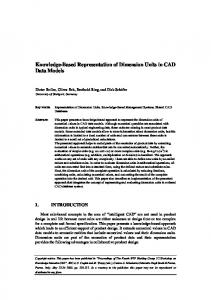
Fig. 1. Atlas creation algorithm

depend on the choice of a single group member as a target for registrations of the remaining images [4]. In this case the average image is crisp as a result of highly resolved morphological matching, but the common space is biased toward the target brain. To this end, an excellent advancement in reducing the impact of such biasing is proposed in [4]. The work of [7] is an interesting compromise between these two extremes, because they derive an optimal common representation using knotpoint based registration (“medium” number of degrees of freedom). A template-free image alignment using the joint image intensity histogram across a group of images was proposed in [8]. This method is best suited for group-wise registration of low-noise, multi-modality images. In this paper we describe a method for groupwise registration which creates both a high-dimensional and unbiased common representation. The output of the algorithm consists of: (i) the average image, as a group average in terms of both image intensities and geometry, and (ii) the variational component, as a set of individual deformation fields that encode the morphological differences between the group average and the individual brains. The variational component captures the distribution of anatomical locations across the group. By making an analogy with one-dimensional measurements, we can say that the average image represents an estimate of the sample mean, while magnitudes of the deformation vectors in the variational component can be used to estimate “error bars” (spheres) for anatomical locations. We demonstrate the algorithm on a set of 27 high resolution mouse brain MR images.

Deformation Based Representation of Groupwise Average and Variability

2

617

Atlas Creation Algorithm

The input to the algorithm is a set of n images denoted I1 , . . . , In . The algorithm consists of seven steps which are outlined in Fig. 1. In Step A we define a common affine space. Subsequently, individual images are resampled into this common space and intensity normalized. At the end of Step A, only extrinsic and anatomically insignificant differences are removed. The following five steps (N1N5) assume nonlinear registration models with increasing levels of resolution. Each nonlinear registration step uses the average image of the previous step as the source. The common average nonlinear space evolves iteratively until a fully resolved groupwise alignment is reached. Finally, in Step C, the common space is geometrically centered with respect to the affinely normalized images. The details are given next. Step A (Affine spatial normalization). We start by performing all pairwise affine registrations among the input images. We use a full affine (12 parameter) model with Levenberg-Marquardt minimization of the ratio image uniformity cost function [12]. The unbiased common affine space is defined by matrix averaging and reconciliation [13]. Each individual image Ik is transformed into this common space and is denoted Jk . In order to ensure unbiased intensity averaging, we first perform intensity normalization of images J1 , . . . , Jn . We begin by correcting image intensity nonuniformity using the method of [10]. We then apply the method of [6] to estimate the mean gray matter intensity in all images. The images are subsequently normalized to the average mean gray matter intensity using linear intensity rescaling. Images thus produced represent spatially (via an affine transformation model) and intensity normalized versions of the initial raw images and are denoted P10 , . . . , Pn0 . The initial average image P0 is created as their voxel-byvoxel intensity average. Steps N1-N5 (Nonlinear spatial normalization). The structure of all nonlinear steps is the same: in Step Ni, the output individual images from the previous step, P1i−1 , . . . , Pni−1 , are registered with the most recent average image Pi−1 (the intensity average of P1i−1 , . . . , Pni−1 ). The nonlinear registration optimizes a similarity function based on a cross-correlation statistic within local neighborhoods which are centered on a regular grid [2]. The nonlinear steps of the algorithm are scheduled in a multi-resolution/multi-scale fashion. The resolution refers to the grid resolution measured by nodal distances. In conjunction with grid resolution, the similarity function is evaluated for extracted image features at appropriate scales (gaussian blur and/or gradient magnitude). Step N1, for example, uses two levels of resolution, first based on 12-voxel grid (nodal distance = 12 voxels in each direction) and second on a 10-voxel grid. The final resolution in Step N5 is maximal, i.e., the grid density equals the image resolution (nodal distance = 1 voxel). The parameters of the multi-resolution schedule have been initially selected similarly as in [2], and then experimentally optimized for maximum registration accuracy and robustness. Full details are given in Table 1.

618

N. Kovacevic et al.

Step C (Centering). A desirable property of any common space is to be minimally distanced from all group members [5]. If gk denotes the cumulative transform of Steps N1-N5 so that Pk5 = gk (Pk0 ) then the corresponding inverse transforms gk−1 are vector fields originating in the same space, that of P5 . The average inverse transform G is defined as G(x) =

1
−1 gk (x), x ∈ P5 . n

(1)

k

By composing transforms we define Fk = G ◦ gk and corresponding images Pk = Fk (Pk0 ), k = 1, . . . , n. Their voxel-by-voxel intensity average image P is our final average image. By construction, the space of P is at the centroid position with respect to P10 , . . . , Pn0 . The set of inverse transforms F−1 k represents the variational component; as vector fields, they originate in the P-space and transform into affinely normalized individual images. For any anatomical location x ∈ P, the distribution of the homologous locations across individual images is given by {F−1 k (x)}k=1,...,n . Table 1. Schedule of nonlinear registrations in Steps N1-N5. The middle column represents grid resolutions in terms of the nodal distance. The right column lists feature extracted images used in each step; the feature scales are measured by the size of the convolving Gaussian kernels, measured in voxels Grid resolution Step Step Step Step Step Step Step Step Step Step

3

N1.1 N1.2 N2.1 N2.2 N3.1 N3.2 N4.1 N4.2 N5.1 N5.2

12 10 8 6 4 3 3 2 2 1

Gaussian fwhm/feature 4/blur 4/gradient 3/blur 3/gradient 3/blur 3/gradient 2/blur 2/gradient 2/blur 2/gradient

magnitude magnitude magnitude magnitude magnitude

Experimental Validation

We demonstrate the algorithm on the set of n = 27 MR images of excised mouse brains with different genetic backgrounds. The animals were selected from three well established mouse strains, 129SV, C57BL6 and CD1, with 9 animals per strain. In vitro imaging was performed using a 7.0-T, 40-cm bore magnet with modified electronics for parallel imaging [1]. The parameters used were as follows: T2-weighted, 3D spin-echo sequence, with TR/TE = 1,600/35 ms, single average, F OV = 24 × 12 × 12 mm and matrix size = 400 × 200 × 200 giving an image

Deformation Based Representation of Groupwise Average and Variability

619

with (60 µm)3 isotropic voxels. The total imaging time was 18.5 hrs. The atlas creation algorithm has been applied to the entire data set. The progression of the algorithm can be observed in gradual sharpening of the average image updates (Fig. 2). This shows how groupwise consensus has been achieved with an increasing level of detail. In fact, the final average image is so well delineated in all major structures (e.g., corpus callosum, fimbria of the hippocampus, anterior commissure) that it surpasses any of the individual images. This effect is similar to the improvement in signal-to-noise ratio in the case when several images of the same subject are averaged together. In this experiment, however, the input images have significantly different morphologies, which means that a high level of delineation in the average image is due to excellent groupwise registration. Two exceptions to this rule are: small and highly variable internal structures (diameter < 120 µm = 2 voxels, e.g., blood vessels, striatal white matter tracks) and the outer brain surface where unresolved differences remain due to inconsistencies in sample preparation and imaging.

Fig. 2. Examples of individual and average images. Top row: images of 3 different individual mouse brains after global affine normalization. Bottom row: average image updates at different stages of the algorithm.)

The variability of the group in terms of the local morphological differences is captured by the variational component: for each P -voxel, there are n = 27 deformation vectors, each consisting of 3 spatial components. In order to summarize and visualize this vast amount of data (∼ 5 GB, assuming floating point

620

N. Kovacevic et al.

representation) we estimate the standard deviation of deformation magnitudes (SDDM ) within the average space:  1
SDDM (x) = ||x − Fk−1 (x)||2 , x ∈ P. (2) n−1 k

In other words, SDDM can be treated as an “image” in the same spatial domain as P , such that the voxel intensities represent distances. By displaying the SDDM image in conjunction with the average image, we are able to classify anatomical regions according to the spatial variability (Fig. 3). The highest variability (SDDM values up to ∼ 900 µm) is found in the olfactory bulbs and at the posterior end of the brain stem. This is expected because these regions are most affected by the inconsistencies in sample preparation. For the rest of the brain, the average SDDM value is 183 µm. Among interior regions, the most variability is found in the ventricles, corpus callosum, fimbria of the hippocampus and far branches of arbor vita.

Fig. 3. Morphological variability of the group. Average image (left), SDDM image (middle) and overlay (right)

While the full validation of the methodology is outside the scope of this paper, we present two experiments in this direction. The first one is a cross-validation for the average SDDM , based on the a priori known genetic background of the samples. For this purpose we created six sub-atlases, each based on 9 images. A sub-atlas is obtained by running the algorithm on the selected image subset only. Each sub-atlas has its own geometrically centered average image and variability component. The first 3 sub-atlases were created to represent a single mouse strain. The other 3 sub-atlases were created by randomly selecting 3 subjects from each of the three strains, totaling to 9 subjects. The variability of the subatlases is evaluated using the average SDDM measure. The results are given in Table 2. They confirm the expectation that pure strain atlases have significantly smaller variability than any of the mixed ones. Also, the variability of the mixed sub-atlases is approximately the same as the variability of the full mixed atlas, as it should, since the weights of the three strains within each mixed sub-atlas are the same as in the full atlas. These result indicate that the variabilty estimate is sensitive to group hetreogenity and inter-group differences. In the second validation experiment we examined atlas bias, rather than registration accuracy. We started with a single brain image, resampled to (120 µm)3

Deformation Based Representation of Groupwise Average and Variability

621

Table 2. Average SDDM value of the full atlas and 6 sub-atlases (in µm) Full mixed 129SV C57BL6 CD1 mixed1 mixed2 mixed3 183

158

145

127

173

180

184

resolution, and 70 regularly spaced landmarks. We used a Gaussian random noise model to displace the landmarks and deform the image in 40 different ways, using thin-plate splines. In addition, we applied random Gaussian noise (8% of the mean brain signal) to image intensities of the 40 deformed images. The resulting images represent a sample with a known mean shape and a known shape variation (with ∼ 5 voxels mean displacement over all landmarks and brains). We applied our algorithm to these 40 images in order to measure how accurately it calculates the average shape. For each landmark and each synthetic image we calculated the distance between the known deformation into the space of the sample mean to the calculated deformation into the average space produced by the algorithm. The average distance between the two target positions, across all landmarks and all brains, was found to be 110 µm. This means that the true mean shape and the one recovered by the algorithm are identical, up to a subvoxel distortion on average.

4

Conclusions

We have developed a methodology for creating an unbiased nonlinear average model from a group of images. There is no dependence on a particular member of the group, and at the same time, the groupwise registration is highly resolved, as demonstrated in the Experimental Validation. The novelty of our approach lies in using an evolving intensity average image as the source for nonlinear registrations with the individual images. In this way we avoid problems associated with attempts to fully localize anatomical differences of the group members with respect to a single individual. Instead, we use a multi-resolution strategy to gradually refine the group-wide consensus. The space of the average image is constructed so that every anatomical location lies at the centroid of the homologous locations across the individual group members. Therefore, the SDDM of deformation magnitudes can be used as a measure of local spatial variability. We have shown that the average SDDM value across the brain can be used as a robust global variability estimate. The methodology presented here has several implications within the general context of deformation based morphometry. For example, atlases based on normal populations can be used for the detection and characterization of abnormal/pathological deviations. Such questions are particularly interesting in the context of mouse phenotyping, where the power of detection becomes greatly amplified through the use of strictly controlled, genetically uniform populations. Furthermore, there is a clear potential for inter-group comparisons. To this end, population or disease specific atlases can be constructed and compared using

622

N. Kovacevic et al.

registration. The deformation field that warps one atlas onto another can then be parsed for significant deformations, i.e., those that surpass the variational components of the two atlases. Acknowledgments. This work was supported by the Canada Foundation for Innovation, the Ontario Innovation Trust and the Burroughs Wellcome Fund. The authors would like to thank Nir Lifshitz for technical assistance.

References 1. N.A. Bock, N.B. Konyer and R.M. Henkelman: Multiple-mouse MRI. Magn. Res. Med. 49 (2003) 158-167 2. D.L. Collins and A.C. Evans: Animal: Validation and applications of non-Linear registration-based segmentation. Int. J. Pattern Recogn. 11 (1997) 1271-1294 3. A.C. Evans, W. Dai, D.L. Collins, P. Neelin and S. Marrett: Warping of a computerized 3D atlas to match brain image volumes for quantitative neuroanatomical and functional analysis. SPIE Medical Imaging 1445 (1991) 236-247 4. A. Guimond, J. Meunier and J.P. Thirion: Average brain models: a convergence study. Comput. Vis. Image. Und. 77 (2000) 192-210 5. P. Kochunov, J.L. Lancaster, P. Thompson, R. Woods, J. Mazziotta, J. Hardies and P. Fox: Regional spatial normalization: Towards an optimal target. J. Comput. Assist. Tomogr. 25 (2001) 805-816 6. N. Kovacevic, N.J. Lobaugh, M.J. Bronskill, B. Levine, A. Feinstein and S.E. Black: A robust method for extraction and automatic segmentation of brain images. Neuroimage 17 (2002) 1087-1100 7. S. Marsland, C.J. Twining and C.J. Taylor: Groupwise non-rigid registration using polyharmonic clamped-plate splines. MICCAI (2003) LNCS 2879 771-779 8. C. Studholme: Simultaneous Population Based Image Alignment for Template Free Spatial Normalisation of Brain Anatomy. WBIR (2003) LNCS 2717 81-90 9. J.C. Mazziotta, A.W. Toga, A.C. Evans, P. Fox and J. Lankaster: A probabilistic atlas of the human brain: theory and rationale for its development. Neuromiage 2 (1995) 89-101 10. J.G. Sled, A.P. Zijdenbos and A.C. Evans: A nonparametric method for automatic correction of intensity nonuniformity in MRI data. IEEE Trans. Med. Imaging 17 (1998) 87-97 11. P.M. Thompson, A.W. Toga: A Framework For Computational Anatomy. Comput. Visual. Sci. 5 (2002) 13-34 12. R.P. Woods, S.T. Grafton, C.J. Holmes, S.R. Cherry and J.C. Mazziotta: Automated Image Registration: I. General methods and intrasubject, intramodality validation. J. Comput. Assist. Tomogr. 22 (1998) 139-152 13. R.P. Woods, S.T. Grafton, J.D.G. Watson, N.L. Sicotte and J.C. Mazziotta: Automated Image Registration: II. Intersubject validation of linear and nonlinear models. J. Comput. Assist. Tomogr. 22 (1998) 153-165