Degree- and Time-Constrained Broadcast Networks
Michael J. Dinneen Department of Computer Science, University of Auckland, Auckland, New Zealand Geoffrey Pritchard Department of Statistics, University of Auckland, Auckland, New Zealand Mark C. Wilson Department of Mathematics, University of Auckland, Auckland, New Zealand
We consider the problem of constructing networks with as many nodes as possible, subject to upper bounds on the degree and broadcast time. This paper includes the results of an extensive empirical study of broadcasting in small regular graphs using a stochastic search algorithm to approximate the broadcast time. Significant improvements on known results are obtained for cubic broadcast networks. © 2002 Wiley Periodicals, Inc. Keywords: broadcast networks; bounded degree; diameter; girth; Cayley graphs
1. INTRODUCTION Broadcasting is the process of sending a message originating at one node of a network to all other nodes, with the restriction that each node can only forward the message to one of its neighbors at a time. In other words, this is the familiar telephone (or point-to-point) communication model. For a comprehensive survey of this and other communication models, see [10]. The classic broadcast design problem was introduced by Farley and others (see [7]). This is the problem of finding graphs of a given order with the least number of edges such that one can broadcast in minimum time from each vertex. It is easy to observe that the minimum time to broadcast in a network of order n is dlog2 ne, since at each time step the number of vertices that have received
Received May 1, 1998; accepted December 1, 2001 Published online 00 Month 2002 in Wiley InterScience (www. interscience.wiley.com). DOI 10.1002/net.10008 Correspondence to: M. J. Dinneen; e-mail:
[email protected] The third author (M.C.W.) was supported by an NZST postdoctoral fellowship. c 2002 Wiley Periodicals, Inc.
the message can at most double. The current state of this broadcast problem is presented in [6]. Formally, a broadcast protocol for a vertex v (called the originator) of a graph G = (V, E) may be defined as follows: It is a sequence V0 = {v}, E1 , V1 , E2 , . . . , Et , Vt = V such that each Vi ⊆ V, each Ei ⊆ E, and for 1 ≤ i ≤ t, 1. Each edge in Ei has exactly one endpoint in Vi−1 , 2. No two edges in Ei share a common endpoint, and 3. Vi = Vi−1 ∪ {w | {u, w} ∈ Ei }.
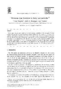
Here, Vi is the set of vertices which have been informed after i steps. During time step i, each vertex in Vi \Vi−1 receives the message from a unique vertex in Vi−1 and each informed vertex in Vi−1 sends to at most one uninformed neighbor. The broadcast time for a vertex v of G, denoted b(G, v), is the minimal length t of a broadcast protocol for v. The broadcast time of the graph G is b(G) = max(b(G, v) | v ∈ G). This paper focuses on the broadcasting problem from a slightly different perspective. Instead of fixing the order and minimizing the number of edges, we constrain both the degree ∆ and the broadcast time T while maximizing the order. A (∆, T) broadcast graph is a graph G such that (1) the degree of every vertex v ∈ V(G) is at most ∆ and (2) the broadcast time of G is at most T. We define B(∆, T) [respectively, Btr (∆, T)] to be the maximum number of vertices possible for a graph (respectively, a transitive graph) with maximum degree ∆ and broadcast time T. Two examples of (3, 4) broadcast graphs of order 14 are given in Figure 1. One broadcast protocol is indicated for the symmetric Heawood graph by labeling the edges with the transmission times. The nonsymmetric graph on
NETWORKS, Vol. 39(3), 121–129 2002 ID Line:
March 11, 2002, 11:39am
W-Networks (39:3) 8u3e1019
FIG. 1. Two different (3, 4) broadcast graphs.
the right requires three different broadcast protocols (one for each white/black/gray node). The degree- and time-constrained broadcast problem, also called the (∆, T) problem, was introduced in [4] as an engineering alternative to the previously mentioned broadcast problem of Farley. The (∆, T) problem is related to the degree/diameter network problem. In that situation, the communication model allows a node to simultaneously send a message to all its neighbors in one time step (the multicast model). Network designers want the largest possible architecture that satisfies the physical constraints on the number of connections per processor (degree) and limitations on overall communication time (diameter). In the classic broadcast problem, it is observed that these sparse graphs often have a few vertices of very high degree, making networks modeled on these graphs impractical. We say that a (∆, T) broadcast graph G is optimal if |V(G)| = B(∆, T). It is trivial to see that the cycle C2T is optimal for ∆ = 2 and T ≥ 2. However, for ∆ ≥ 3, the (∆, T) problem is decidedly nontrivial. The main reason is that, in general, the problem of computing the broadcast time of a given graph is very difficult. It is straightforward to reduce the instances of the three-dimensional matching problem to a corresponding minimum broadcast time problem and thereby prove NPcompleteness for the general case of unbounded-degree networks [8]. A simple proof showing that the problem of finding the broadcast time of networks of maximum degree 3 is NP-complete was presented in [3]. A more involved proof by Middendorf [12] shows that, in the context of broadcasting with multiple originators in cubic planar graphs, even the problem of determining whether the broadcast time is at most 2 is NP-complete. Since exact algorithms are impractical for large networks, several heuristics have been proposed (e.g., see [11, 15, 19]). Also, because of the general hardness of this problem, some research has been restricted to specific families of “nice” graphs. For example, a near-optimal broadcasting
122
algorithm for the pancake graphs, a family of Cayley graphs, was given in [9]. The difficulty of exhibiting broadcast protocols (evident even in the second graph in Fig. 1) is one reason for concentrating on transitive (also called vertex-transitive or vertex-symmetric) graphs. By definition, each vertex of such a graph G may be mapped to any other vertex by a suitable automorphism of the graph [in other words, the automorphism group Aut(G) acts transitively on V(G)]. Hence, it suffices to find a protocol for a single originator instead of one for each possible originator. An important subclass of transitive graphs is the class of Cayley graphs. Recall that, given a group (G, ·) and a set S of generators of G which is closed under inverses, the Cayley graph Γ = Cay(G, S) is defined by V(Γ) = G and E(Γ) = {{x, x · s} | x ∈ G, s ∈ S}. Cayley graphs, because of their accessibility and their transitivity properties, have been systematically and successfully used to model many of the largest known degree/diameter networks (e.g., see [5, 17]). Thus, an investigation of these graphs is a natural starting point in an attempt to establish lower bounds for the (∆, T) problem. An outline of the paper follows: In Section 2, we present the best lower bounds known for B(∆, T) and Btr (∆, T), for small values of ∆ and T. We discuss explicit examples of graphs which achieve these bounds. Section 3 contains various necessary conditions on (∆, T) networks, including some upper bounds on B(∆, T) and Btr (∆, T). Some further graph constructions, establishing lower bounds on B(∆, T) and Btr (∆, T), appear in Section 4, including a result on the asymptotic behavior of B(∆, T) as T → ∞. Section 5 contains comments on our methodology and Section 6 finishes with a list of selected open problems. We end this Introduction by mentioning two more broadcasting problems related to the (∆, T) problem, neither of which we studied in this paper. Both of these place limits on the broadcast time but have no degree constraints (as they were originally proposed). One variation of the time-constrained broadcasting problem is the bounded depth broadcasting problem of
NETWORKS–2002
ID Line:
March 11, 2002, 11:39am
W-Networks (39:3) 8u3e1019
Peters and Peters [13], where there is a limit on the number of times information can be retransmitted before it becomes unusable. They defined a (t, d)-broadcast graph to be a graph in which broadcasting can be completed from any originator in time t and depth d. Another time-restricted broadcasting problem was introduced by Shastri [18], where the goal was to find the sparsest networks of order n with broadcast time slightly more than the minimum time. Here, a t-relaxed minimal broadcast network G is a network in which broadcasting can be accomplished in dlog2 v(G)e + t time units from any node. It turns out that for relatively small t the sparsest networks are trees, so this parameterized problem is probably not of much interest to engineers. 2. NUMERICAL RESULTS In this section, we present the best-known lower bounds on B(∆, T) for small values of ∆ and T and explicitly present graphs attaining these bounds. For ∆ > 2, there are only two infinite families of graphs which are known to be optimal for the (∆, T) problem. For T = ∆, the hypercube Q∆ [the Cayley graph of (Z2 )∆ with respect to the standard generating involutions] is optimal. For T = ∆ + 1, the Cayley graph ∆ of the dihedral group D2∆−1 −1 = ha, b | a2 = b2 −1 = 2 2i −1 |0≤i≤ (ab) = 1i, with respect to generators {ab ∆ − 1}, is optimal (see [4]). In each of these cases, a protocol exists which is as simple as possible. Specifically, there is an ordering s0 < s1 < · · · < s∆−1 of the set of generators such that at time step i vertex x sends to vertex xsj , where 0 ≤ j ≤ ∆ − 1 and j ≡ i mod ∆. In other words, at a given time step, all transmissions are in a fixed “dimension” and these dimensions cycle through the elements of S. We shall call such a protocol a simple protocol. We believe that simple protocols are rather rare among graphs that are close to optimal for this problem.
We now present our numerical results. Details of our methodology are delayed until Section 5. Table 1 presents the best-known lower bounds on B(∆, T) for small values of ∆ and T, T ≥ ∆ ≥ 3. In Table 1, bold entries are known to be optimal. All these, in fact, attain the upper bound on B(∆, T) given in Table 2. Italicized entries are new results. All entries in Table 1 were obtained explicitly from Cayley graphs unless indicated by a superscript. An asterisk (∗ ) indicates that the entry is transitive but not a Cayley graph, while a dagger (†) means that the entry is obtained from a compound construction as explained in Section 4. We note that, while it is possible that B(3, 7) = 66, so that the (3, 7) entry need not be optimal, it can be shown that Btr (3, 7) = 64 (since all cubic transitive graphs of order 66 are known and can be eliminated by the methods of Section 3). For comparison, we have included, in Table 2, some upper bounds on B(∆, T). For the origin of these bounds, see Section 3. Table 3 shows the properties of the largest cubic broadcast graphs for T ≤ 12. All these graphs are transitive. In brackets, we list how many nonisomorphic graphs that we found of the given order. For comparison, we list, in the third column, the order of the largest-known cubic (transitive) graph with diameter T. We believe that our bounds for diameters T = 6 and T ≥ 10 are new (see Appendix A of [20]). In the remaining columns, we state properties of what we considered to be the “best” one of the broadcast graphs obtaining the broadcast time T. This is often a symmetric graph, that is, Aut(G) is transitive on the set of directed edges. In addition, each best broadcast graph is bipartite (many of the others are not). We now discuss our new entries in Table 1 in more detail (see [4] for previous details). (3, 5): There are exactly four cubic transitive graphs with 24 vertices and broadcast time 5, all of which are Cayley graphs. Of these, we discuss two in more detail. For the first, let G be the symmetric group S4 and let S =
TABLE 1. Orders of the largest-known broadcast networks with degree ≤ ∆ and broadcast time ≤ T.
NETWORKS–2002 123 ID Line:
March 11, 2002, 11:39am
W-Networks (39:3) 8u3e1019
TABLE 2. Upper bounds on B(∆, T).
{s0 , s1 , s2 } = {(13), (14), (12)(34)} ⊂ G. Then, the graph Γ = Cay(G, S) has a simple protocol with the generators taken in the given order. The second graph is the unique symmetric graph of this order and does not have a simple protocol. (3, 6): There is a unique cubic transitive graph Γ with 40 vertices and broadcast time 6. Γ is also the unique cubic symmetric graph of order 40 and is not a Cayley graph. It differs from the (3, 6)-graph of order 40 presented in [1], which is not even transitive. (3, 7): There are exactly six cubic transitive graphs with 64 vertices and broadcast time 7. One of these has diameter 6. Among these is the unique symmetric graph of this order. This graph Γ occurs as the Cayley graph of four nonisomorphic groups of order 64. (3, 8): We found a cubic Cayley graph Γ with 96 vertices and broadcast time 8, and there are at most 14 such graphs. Γ is not symmetric. One description of Γ as Cay(G, S) is as follows: The group G is the semidirect product C × | D16 , where D16 is generated by involutions a, b subject to (ab)16 = 1 and their action on a
generator t of the cyclic group C of order 3 is given by ata−1 = t, btb−1 = t−1 . We can take S = {a, b, (ab)3 at}. (3, 9): We found three cubic Cayley graphs with 144 vertices and broadcast time 9. One such is the Cayley graph of the group G = ha, b | a2 = ab4 ab−4 = (b2 ab)3 = (abab2 )2 = 1i, with respect to {a, b, b−1 }. (3, 10): We found three cubic Cayley graphs with 216 vertices and broadcast time 10. Among these is one of the three symmetric graphs of this order, known as F216C in the Foster Census (see [16]). (3, 11): We found two cubic Cayley graphs with 324 vertices and broadcast time 11, neither of which is symmetric. One such is the Cayley graph of G = ha, b, c | a2 = b2 = c2 = cbacabacabca = 1, (cab)2 = (bca)2 i, with respect to {a, b, c}. (3, 12): We found a cubic Cayley graph with 506 vertices and broadcast time 12. One representation is Cay(G, S), where G is the semidirect product Z23 ×| Z22 . The action is determined by the requirement that the generator 1 ∈ Z22 maps to the generator 5 ∈ Z∗ 23 Aut(Z23 ). We can take S to be the set {(1, 21), (18, 1), (0, 11)} ⊂ Z23 × Z22 .
TABLE 3. Vital statistics of the largest-known cubic broadcast networks. General transitive lower bounds
Properties of best broadcast graph
T
Max|V|(b(G) = T) broadcast graph
Max|V|(diam(G) − T) multicast graph
Girth
Diameter
|Aut|
Symmetric?
3 4 5 6 7 8 9 10 11 12
8 [2] 14 [1] 24 [4] 40 [1] 64 [6] 96 [1] 144 [3] 216 [3] 324 [2] 506 [1]
14 30 60 82 168 300 506 882 1220 1830
4 6 6 8 8 10 10 12 12 14
3 3 4 6 7 7 8 8 9 9
48 336 144 480 384 96 288 1296 324 506
Yes Yes Yes Yes Yes No No Yes No No
124
NETWORKS–2002
ID Line:
March 11, 2002, 11:39am
W-Networks (39:3) 8u3e1019
(4, 6): There is a degree 4 transitive graph Γ of order 56 and broadcast time 6 which was presented in [1]. A broadcast protocol was given in that paper. Γ may be represented as a Cayley graph of D28 = ha, b | a2 = b28 = (ab)2 = 1i, with respect to the set of generating involutions {a, ba, b9 a, b26 a}. All other new entries which we have found are Cayley graphs similar to the description of the (3, 12) entry. The groups are all semidirect products of two cyclic groups Zm ×| Zn . In Table 4, the triple (m, n, k) indicates that the homomorphism from Zn into Z∗ m Aut(Zm ) is determined by the requirement that it map the generator n 1 of Zn to an element k ∈ Z∗ m such that k = 1. The ordered pairs represent the ∆ generators of the Cayley graph in the usual way as elements of the set Zm × Zn . The group multiplication in Zm ×| Zn , which is usually noncommutative, of the elements (m1 , n1 ) and (m2 , n2 ) is the element (m1 + kn1 · m2 , n1 + n2 ). 3. UPPER BOUNDS In this section, we derive upper bounds on the size of a (∆, T) graph in terms of easily computable graphtheoretic properties of the graph. These results help us eliminate many potential candidates while searching for large (∆, T) graphs. Let Γ(d) be the infinite rooted tree in which every vertex has d children. Then, Γ(d) has an obvious broadcast protocol from the root, in which every vertex sends to its children in turn (in some specified fixed order). For each t ≥ 0, let Γ(d, t) be the subtree of Γ(d) consisting of all vertices which have received the message after t time steps. More immediately relevant to broadcasting is Γ0 (d), the infinite rooted tree in which every vertex has degree d (so the root has d children and all other vertices have d − 1 children). Define Γ0 (d, t) analogously to Γ(d, t): the vertices informed after t broadcast steps. Throughout this section, we will assume d ≥ 2 for Γ(d) and d ≥ 3 for Γ0 (d) in order to avoid trivial cases. Let F(d, t) be the number of vertices of Γ(d, t), let f(d, t, k) be the number of vertices of Γ(d, t) of depth at most k, and let g(d, t, k) = F(d, t) − f(d, t, k) be the number of vertices of Γ(d, t) of depth greater than k. Define analogous quantities F0 , f0 , g0 for Γ0 (d). The following easily established equations are useful in calculating the above quantities: Proposition 3.1. The following relations hold for the above values of d. The function F satisfies the recurrence F(d, 0) = 1,
F(d, T) = 1 min(d,T) X F(d, T − i) +
for T ≥ 1.
i=1
The function F0 is given by F0 (d, T) = 2F(d − 1, T − 1).
The function f satisfies the recurrence f(d, T, k) Pmin(d,T) f(d, T − i, k − 1), 1 + i=1 if T ≥ 1 and k ≥ 1 = 1, if T = 0 or k = 0. The function f 0 is given by f 0 (d, T, k) = f(d−1, T−1, k)+f(d−1, T−1, k −1). If a graph G has maximum degree ∆ and a broadcast protocol of time T originating from a vertex v0 , then this protocol induces a broadcast tree (the subgraph S of G on the same vertex set, incorporating only those edges used in the broadcast). Of course, S is a tree rooted at v0 . We may also view S as a subtree of Γ0 (∆, T) in an obvious way. Thus, F0 (∆, T) provides an upper bound for B(∆, T). This argument is the basis of the table of upper bounds for B(∆, T) given earlier. The next result extends this kind of counting argument still further, to obtain a useful method for bounding the broadcast times of particular graphs. Proposition 3.2. Let G be a graph with maximum degree ∆ and broadcast time T. Let v0 be a vertex of G. Then, for 0 ≤ k ≤ T, |{vertices w of G | ρG (v0 , w) > k}| ≤ g0 (∆, T, k). Here, ρG denotes the usual graph-theoretic distance metric on the vertex set of G. Proof. Let S be a broadcast tree for G with originator v0 and time T. Note that for any vertices v, w of G we have ρG (v, w) ≤ ρS (v, w). Then, |{vertices w of G|ρG (v0 , w) > k}| ≤ |{vertices w of S|ρS (v0 , w) > k}| ≤ |{vertices w of Γ0 (∆, T)|ρΓ0 (∆,T) (v0 , w) > k}| = g0 (∆, T, k). For the last step, we have viewed S as a subtree of Γ0 (∆, T). If we apply the above result with k = T, we recover the obvious fact that b(G) ≥ diam(G), that is, the diameter of a graph may not exceed its broadcast time. We now move on to consider what effect the girth (the length of the smallest cycle) of a graph has on its broadcast time. Intuitively, for regular graphs of degree d, one expects that large trees Γ0 (d, T) cannot be embedded in a graph G if the root is to lie in a small cycle of G. The next result makes this idea precise. Let β(∆, g, T) be the maximum number of vertices among all graphs Γ with maximum degree ∆, girth g, and broadcast time T, and let βtr (∆, g, T) denote the same function restricted to the transitive graphs.
NETWORKS–2002 125 ID Line:
March 11, 2002, 11:39am
W-Networks (39:3) 8u3e1019
TABLE 4. Data for Cayley graphs of semidirect products of cyclic groups. (∆, T)
(m, n, k)
(4, 7) (4, 8) (4, 9) (4, 10) (4, 11) (4, 12) (5, 7) (5, 8) (5, 9) (5, 10) (5, 11) (5, 12) (6, 8) (6, 9) (6, 10) (6, 11) (6, 12) (7, 9) (7, 10) (7, 11) (7, 12) (8, 10) (8, 11) (8, 12) (9, 11) (10, 12)
(24, 4, 5) (27, 6, 2) (17, 16, 3) (31, 15, 3) (97, 8, 5) (85, 16, 3) (29, 4, 2) (35, 6, 2) (13, 30, 2) (49, 14, 3) (86, 14, 3) (136, 16, 3) (13, 18, 2) (44, 10, 3) (35, 24, 2) (69, 22, 2) (117, 24, 2) (27, 18, 2) (17, 56, 3) (73, 24, 5) (113, 28, 3) (50, 20, 3) (73, 27, 5) (43, 84, 3) (101, 20, 2) (145, 28, 2)
Generators (23, 2), (1, 2), (17, 3), (11, 1) (10, 3), (15, 4), (12, 2), (0, 3) (5, 7), (15, 9), (7, 11), (16, 5) (4, 8), (22, 7), (5, 4), (23, 11) (86, 5), (65, 3), (79, 4), (0, 4) (39, 11), (43, 5), (80, 14), (45, 2) (20, 2), (13, 2), (26, 1), (22, 3), (0, 2) (12, 3), (2, 3), (19, 2), (1, 4), (0, 3) (10, 22), (9, 8), (12, 6), (1, 24), (0, 15) (6, 1), (27, 13), (46, 12), (31, 2), (0, 7) (7, 2), (25, 12), (5, 6), (49, 8), (0, 7) (131, 15), (15, 1), (54, 9), (86, 7), (0, 8) (1, 6), (12, 12), (10, 4), (9, 14), (8, 7), (11, 11) (39, 6), (9, 4), (41, 9), (9, 1), (22, 6), (22, 4) (25, 14), (20, 10), (32, 18), (17, 6), (11, 1), (12, 23) (44, 2), (58, 20), (60, 5), (24, 17), (43, 16), (8, 6) (42, 23), (33, 1), (59, 5), (53, 19), (29, 20), (4, 4) (8, 13), (14, 5), (7, 7), (1, 11), (9, 8), (18, 10), (0, 9) (9, 34), (15, 22), (16, 51), (8, 5), (10, 10), (11, 46), (0, 28) (27, 17), (52, 7), (52, 11), (3, 13), (49, 10), (1, 14), (0, 12) (75, 5), (35, 23), (29, 4), (34, 24), (83, 20), (49, 8), (0, 14) (23, 3), (1, 17), (9, 6), (29, 14), (34, 8), (6, 12), (5, 15), (35, 5) (8, 2), (71, 25), (6, 20), (35, 7), (2, 3), (18, 24), (10, 22), (45, 5) (29, 13), (37, 71), (34, 5), (8, 79), (20, 29), (18, 55), (34, 14), (11, 70) (66, 6), (8, 14), (29, 9), (19, 11), (35, 3), (52, 17), (51, 9), (16, 11), (0, 10) (121, 2), (6, 26), (24, 25), (98, 3), (77, 6), (137, 22), (140, 23), (15, 5), (113, 23), (9, 5)
Proposition 3.3. The following relations hold: if g ≥ T B(3, T), g + F(2, T − 1) β(3, g, T) ≤ + Pg+1 F(2, T − i), if g < T. i=3 βtr (2, g, T) = ( F(2,P T), if 0 ≤ T ≤ g − 1 g g + i=2 βtr (2, g, T − i), if g ≤ T.
It follows from the recurrences given in Proposition 3.1 that, for fixed d, F(d, T) grows as (φd )T as T → ∞, where φd is the unique root in the interval (1, 2) of the polynomial xd+1 − 2xd + 1. This, then, gives an upper bound on the exponential rate of growth of B(∆, T). Note that as d increases φd increases with limit 2. 4. LOWER BOUNDS In this section, we present graph-theoretic constructions which provide general lower bounds for B(∆, T). These results allow one to easily extend Table 1 for larger ranges of ∆ and T. For this current table, ∆ ≤ 10 and T ≤ 12, of the largest-known broadcast graphs, only the lower bound B(9, 12) is generated by one of the combination methods given below.
1. {(u, w), (v, w)}, whenever {u, v} is an edge of G, and 2. {(u, v), (u, w)}, whenever {v, w} is an edge of H.
Proof. Let G1 , G2 be two optimal broadcast graphs for (∆1 , T1 ) and (∆2 , T2 ), respectively. Consider G = G1 ⊗ G2 . It is clear that G has maximum degree at most ∆1 +∆2 . To broadcast in G in time T1 +T2 from an originator (u0 , v0 ), we first take T1 steps to inform all vertices of form (u, v0 ), where u ∈ V(G1 ), using any broadcast protocol which works for G1 . Then, beginning from each (u, v0 ), take T2 steps to inform all vertices (u, v), where v ∈ V(G2 ), using any protocol which works for G2 . Corollary 4.3.
B(∆ + 1, T + 1) ≥ 2B(∆, T).
Proof. In Proposition 4.2, take one of the graphs to be K2 , the graph with two vertices and one edge. Corollary 4.4.
For k ≥ 2, B(∆ + 2, T + k) ≥ 2kB(∆, T).
Proof. In Proposition 4.2, take one of the graphs to be C2k , the cycle of length 2k.
Combination Methods In this subsection, we explore some ways of con-
126
Definition 4.1. Given two graphs G and H, the compound product G ⊗ H has vertex set V(G) × V(H) and edges:
Proposition 4.2. B(∆1 +∆2 , T1 +T2 ) ≥ B(∆1 , T1 )B(∆2 , T2 ).
βtr (3, g, T) = 2βtr (2, g, T − 1).
4.1.
structing graphs with good broadcast times out of smaller graphs with good broadcast times. Initially, we consider the possibility of compounding two graphs.
Proposition 4.5.
B(∆ + 1, T + 3) ≥ 4B(∆, T).
NETWORKS–2002
ID Line:
March 11, 2002, 11:39am
W-Networks (39:3) 8u3e1019
Proof. Let G be an optimal broadcast graph for (∆, T). Since G is connected, we may take a spanning tree of G and use it to characterize every vertex of G as even or odd, according to its distance from the root. Let G0 = G ⊗ C4 . (As usual, the vertex set of the cycle C4 is taken to be Z4 and the edge set {{x, y} | y = x + 1}.) For each even vertex v of G, delete from G0 the edges between (v, 0) and (v, 1) and between (v, 2) and (v, 3). For each odd vertex v of G, delete from G0 the edges between (v, 1) and (v, 2) and between (v, 3) and (v, 0). Thus, G0 has maximum degree at most ∆ + 1. To broadcast in G0 from an originator (v, x), proceed as follows: At the first step, inform (v, y), where y = x ± 1 depending on the parity of v. At the second step, inform (w, x) and (w, y), where w is a neighbor of v with the opposite parity to v. At the third step, we can inform (w, z1 ) and (w, z2 ), where z1 and z2 are such that {x, y, z1 , z2 } = Z4 . The remainder of the broadcast can be accomplished by applying the original protocol for G to the sets {(v, t) | v ∈ v(G)}, where t = x, y, z1 or z2 . We conjecture that B(∆ + 1, T + 2) ≥ 3B(∆, T). This is almost shown by the next result, which requires one extra hypothesis. Definition 4.6. A graph G is pairable if it has a 1regular subgraph which includes all the original vertices. Such a subgraph connects the vertices of G into pairs (such pairings are also called 1-factorizations or perfect matchings). Proposition 4.7. Let G be a pairable graph with maximum degree at most ∆ and broadcast time T. Then, there exists a pairable graph G0 with maximum degree at most ∆ + 1 and broadcast time at most T + 2, and |V(G0 )| = 3|V(G)|. Proof. Let G0 be the disjoint union of three copies of G. If {u, v} is a pair in G, then {(u, i), (v, i)} is a pair in G0 for i = 1, 2, 3. For each such pair, add edges {(u, 1), (v, 2)}, {(u, 2), (v, 3)}, and {(u, 3), (v, 1)}. Now, if the originator is, say, (u, 1), we inform (v, 1) at the first time step and (v, 2) and (u, 3) at the second. The remainder of the broadcast proceeds separately in each of the three copies of G. The maximum degree has increased for all of the methods mentioned so far. To complete this subsection, we give a way of constructing broadcast graphs with lower degree. Definition 4.8. From an adjacency list A, the partial function fA (u, v) is defined to be i if v is the i-th neighbor of u. A two-way split of a graph G = (V, E), with respect to an adjacency list A representation, is a graph H = (V0 , E0 ), where V0 = V × {0, 1} and E0 = E1 ∪ E2 as defined below: E1 = {{(v, 0), (v, 1)} | v ∈ V},
E2 = {{(u, b), (v, c)} | {u, v} ∈ E, b = (fA (v, u) ≤ deg(u)/2) and c = (fA (u, v) ≤ deg(v)/2)}. This splicing idea may be generalized by replacing each vertex with k vertices and partitioning the neighbors evenly into k parts. Instead of using a clique (as was done in the two-way split), the k copies of each of V are connected with a broadcast graph of low degree and small broadcast time. Proposition 4.9.
B(d∆/2e + 1, 2T) ≥ 2B(∆, T).
Proof. From a (∆, T) broadcast graph G of order n, we create a two-way split H of order 2n. The graph H has broadcast time at most 2T by following the broadcast protocols of G. Here, whenever a vertex (v, b) is informed from a vertex (u, c), u ≠ v, a single time-step delay is used to inform (v, 1 − b) before proceeding. 4.2.
A Direct Construction
The cube-connected cycles, introduced by Preparata and Vuillemin [14], are a well-known family of cubic graphs with an underlying hypercubelike structure. Below, we provide a lower bound on the broadcast time of these networks. An immediate consequence of this result is that for all ∆ ≥ 3, B(∆, T) grows exponentially with T. The cube-connected cycles, n-CCC, are similar to the n-cubes. The vertices are given as pairs (i, V), where i ranges between 0 and n − 1 and V is a bit vector of length n. For edges, vertex (i, V) is connected to vertex (i0 , V0 ) if and only if i = i0 and V0 differs in only the i-th bit from V or |i − i0 | = 1 and V = V0 . The cube-connected cycles were shown to be transitive by Carlsson et al. [2]. In fact, they explicitly presented a larger family, the generalized cube-connected cycles, as Cayley graphs. Theorem 4.10. The broadcast time of the cubeconnected cycle(s) d-CCC is at most d(5d − 2)/2e. Proof. Let G be the graph d-CCC. Since G is transitive, we only need to provide one broadcast protocol. We will use an optimal underlying broadcast protocol for the hypercube H of dimension d to construct a broadcast protocol for G. Let C(v) = {(i, v) | i = 0, . . . , d − 1} represent the set of vertices of (cycle of) G that corresponds to a vertex v of H. Note that the set {C(v)|v ∈ V(H)} partitions the vertices of G into equivalence classes. We now describe the broadcast protocol: First, note that we can optimally broadcast in H by using a simple protocol (sending messages to neighbors at dimension t at time t). With vertex (0, 00 · · · 00) as the originator in G, the first broadcast is to vertex (0, 00 · · · 01), that is, we use dimension 1. At time 2, both these vertices send to their first neighbor on the cycle C(v). At time 3, the informed vertices (1, 00 · · · 00) and (1, 00 · · · 01) send to
NETWORKS–2002 127 ID Line:
March 11, 2002, 11:39am
W-Networks (39:3) 8u3e1019
their neighbors in dimension 2. Continue the process as follows: At time step 2t − 1, an informed vertex (t − 1, V) broadcasts in dimension t to its neighbor (t − 1, V + 2t ). There is a transmission delay of one time step after the first vertex of C(v) is informed and before the next neighbor outside of C(v) is informed. Since it takes d time steps to broadcast in the d-cube H, plus d − 1 delays, at least one vertex in each C(v) is informed by time 2d − 1. To finish off the broadcasting in G, we need at most dd/2e time steps for a representative v of C(v) to inform any remaining vertices of the cycle C(v). Thus, we can broadcast in at most 2d −1+dd/2e = d(5d −2)/2e time steps. Corollary 4.11.
B(3, d(5d − 2)/2e) ≥ d2d .
Proof. This result follows from Theorem 4.10 and the fact that d-CCC has d2d vertices. The broadcast bounds given in the previous theorem are not sharp. We found broadcast protocols for the cube-connected cycles 3-CCC and 5-CCC with broadcast times 6 and 11, respectively (one less than our general bound). However, the actual best broadcast time for 4-CCC matches our general bound of 9. On the right of Figure 2, we show a nice broadcast protocol of minimum time for 3-CCC (here, one simply broadcasts clockwise or counterclockwise around each 3-cycle depending on the parity of the time that the first vertex in the cycle receives the message). 5. COMMENTS ON OUR COMPUTATION The examples in Section 2 were generated by examining known graphs with a high degree of symmetry. In particular, the authors found the online database [16] maintained by Royle to be invaluable. The enumeration of transitive cubic graphs in that database was the raw material for Table 3. The generation of random Cayley graphs, based on semidirect products of cycles (see [5]),
was the source of the other ∆-regular graphs that yield new lower bounds in Table 1. Once we have a list of potential graphs, the next requirement is to know their broadcast times. As mentioned in Section 1, finding the broadcast time is very difficult. We were comfortably able to compute broadcast times of cubic graphs with up to about 80 vertices (time T ≤ 8). For graphs of higher degree (∆ ≥ 4), our current tractable range decreases to graphs with fewer than 50 vertices. It is possible to partially overcome this difficulty by using a stochastic search algorithm to find broadcast protocols. We used the following simple rule: At each time step, each informed vertex selects one of its uninformed neighbors at random to inform. This generates a random protocol which will inform the whole graph in some finite time. The process may be repeated as often as desired; the smallest of the times found is an upper bound for the broadcast time of the graph. If this upper bound matches a known lower bound, for a given number of vertices, then we have found the broadcast time of the graph. For the examples given in Section 2, the number of attempted random protocols ranged from a few hundred to a few hundred thousand. Since all of our input graphs were transitive, it was sufficient for our implementation to search for broadcast protocols originating from a single vertex (e.g., in the case of Cayley graphs, we started from the identity vertex). To lessen our computational effort, we explored several results which bound the broadcast time of a graph in terms of easily computable properties, such as the girth and the diameter. The results mentioned earlier in Section 3 were helpful. Proposition 3.2 proved to be an especially sharp test. We observed that graphs with large girth and small diameter often have small broadcast times. This suggests that we should look for graphs with a high girth/diameter ratio. In the cases that we examined, we found that among all transitive cubic graphs on n vertices which pass the tests in Section 3 the minimal broadcast time always occurs for a graph whose girth/diameter ra-
FIG. 2. The cube-connected cycle(s) 3-CCC and two broadcast protocols: (1) via Theorem 4.10; (2) via a minimal broadcast tree.
128
NETWORKS–2002
ID Line:
March 11, 2002, 11:39am
W-Networks (39:3) 8u3e1019
tio is maximal. Another simple heuristic which should work well in practice is to consider graphs with large automorphism groups. We did not use these nonrigorous ideas to eliminate any graphs in our search, but found them accurate enough to mention.
[3] [4]
6. SOME CONJECTURES AND OPEN PROBLEMS Many problems and conjectures arose in the course of this work. We state only a few of them below: •
We know now that B(∆, T) grows exponentially with T for ∆ ≥ 3. It is natural to wonder whether this growth has a limiting exponential rate, that is, whether the quantity f(∆) = lim
T→∞
ln B(∆, T) T
exists. One could also ask what value it takes. The answer might give a succinct, quantitative description of the benefits of higher connectivity (i.e., higher degree). Assume that the limit exists. It is trivial to see that f(2) = 0 and that f(∆) is an increasing function of ∆. We have seen in this paper that f(∆) > 0 for ∆ ≥ 3. The simple estimate B(∆, T) ≤ B(T, T) = 2T gives the upper bound f(∆) ≤ ln 2 for all ∆. The estimates in Section 3 give more √ precise upper bounds; in particular, f(3) ≤ ln((1 + 5)/2) ≈ 0.4812. • All known examples suggest that B(∆, T + 1) ≥ (3/2)B(∆, T). This, if true, would, of course, be a strong lower bound on the actual growth rate of B(∆, T). • Is it true that for all T ≥ 2 there is an optimal (3, T) broadcast graph with girth T+2 if T is even and T+1 if T is odd? • Besides our diameter and girth bounds, does there exist a good polynomial-time algorithm that predicts whether a graph has a small broadcast time?
[5] [6]
[7] [8] [9]
[10] [11] [12] [13] [14] [15]
Acknowledgments
[16]
We thank Golbon Zakeri for inspiring us to continue doing research on the (∆, T) broadcast problem. We also thank Paul Hafner for teaching us how to investigate Cayley graphs with the Magma system and for his comments on an earlier version of this paper.
[17]
REFERENCES
[19]
[1] J.-C. Bermond, P. Hell, A.L. Liestman, and J.G. Peters, Sparse broadcast graphs, Discr Appl Math 36(2) (1992), 97–130. [2] G.E. Carlsson, J.E. Cruthirds, H.B. Sexton, and C.G. Wright, Interconnection networks based on a generaliza-
[18]
[20]
tion of cube-connected cycles, IEEE Trans Comput 34 (1985), 769–777. M.J. Dinneen, The complexity of broadcasting in boundeddegree networks, Technical report LACES-05C-94-31, Los Alamos National Laboratory, 1994. M.J. Dinneen, M.R. Fellows, and V. Faber, “Algebraic constructions of efficient broadcast networks,” Applied algebra, algebraic algorithms and error-correcting codes, Lecture Notes in Computer Science, Springer, Berlin, 1991, Vol. 539, pp. 152–158. M.J. Dinneen and P.R. Hafner, New results for the degree/diameter problem, Networks 24 (1994), 359–367. M.J. Dinneen, J.A. Ventura, M.C. Wilson, and G. Zakeri, Compound constructions of minimal broadcast networks, CDMTCS research report 026, 1997, Discr Appl Math, 93 (1999), 205–232. A.M. Farley, Minimal broadcast networks, Networks 9 (1979), 313–332. M.R. Garey and D.S. Johnson, Computers and intractability. A guide to the theory of NP-completeness, W.H. Freeman, San Francisco, 1979. C. GowriSankaran, Broadcasting on recursively decomposable Cayley graphs, Proc International Workshop on Broadcasting and Gossiping 1990, Sechelt, BC, Canada, Discr Appl Math 53 (1994), 171–182. S.M. Hedetniemi, S.T. Hedetniemi, and A.L. Liestman, A survey of gossiping and broadcasting in communication networks, Networks 18 (1988), 319–349. G. Kortsarz and D. Peleg, Approximation algorithms for minimum-time broadcast, SIAM J Discr Math 8 (1995), 401–427. M. Middendorf, Minimum broadcast time is NP-complete for 3-regular planar graphs and deadline 2, Inform Process Lett 46 (1993), 281–287. D.B. Peters and J.G. Peters, Bounded depth broadcasting, Discr Appl Math 66 (1996), 255–270. F.P. Preparata and J. Vuillemin, The cube-connected cycles: A versatile network for parallel computation, Commun ACM 24 (1981), 300–309. R. Ravi, Rapid rumor ramification: Approximating the minimum broadcast time, Proc 35th IEEE Symp on Foundations of Computer Science, 1994, pp. 202–213. G. Royle, Online graph database at http://www.cs.uwa. edu/∼gordon/. M. Sampels, Large networks with small diameter, Proc 23rd Workshop on Graph-Theoretic Concepts in Computer Science (WG ’97), Lecture Notes in Computer Science, Springer-Verlag, 1997, Vol. 1335, pp. 288–302. A. Shastri, “Broadcasting in general networks. I. Trees,” Computing and combinatorics, Lecture Notes in Computer Science, Springer, Berlin, 1995, Vol. 959, pp. 482–489. P. Scheuerman and G. Wu, Heuristic algorithms for broadcasting in point-to-point computer networks, IEEE Trans Comput 33 (1984), 804–811. L. Twele, Effiziente Implementierung des Todd-Coxeter Algorithmus im Hinblick auf Grad/Durchmesser-Optimierung von knotentransitiven Graphen, Diplomarbeit Universität Oldenburg, 1997.
NETWORKS–2002 129 ID Line:
March 11, 2002, 11:39am
W-Networks (39:3) 8u3e1019