DeLLIS: a Data Mining Process for Fault Localization Peggy Cellier, Mireille Ducass´e, S´ebastien Ferr´e, Olivier Ridoux University of Rennes 1/INSA of Rennes/IRISA ∗ Abstract Most fault localization methods aim at totally ordering program elements from highly suspicious to innocent. This ignores the structure of the program and creates clusters of program elements where the relations between the elements are lost. We propose a data mining process that computes program element clusters and that also shows dependencies between program elements. Experimentations show that our process gives a comparable number of lines to analyze than the best related methods while providing a richer environment for the analysis. We also show that the method scales up by tuning the statistical indicators of the data mining process.
1. Introduction A large amount of information can be collected from program executions , for instance the executed lines, the values of variables or the values of predicates. We call that information the events of the execution, they constitute the execution trace. Fault localization methods that compare execution traces, distinguish two sorts of executions, passed and failed executions. Passed executions behave according to their specification, failed executions do not. These methods are based on the intuition that, firstly, the events that appear only in the traces of failed executions are more likely to be erroneous, and, secondly, the events that appear only in the traces of passed executions are more likely to be innocent. For instance, the nearest neighbor method, by Renieris and Reiss [12], takes into account only one failed execution. A passed execution “near” to the failed execution is then selected. The difference between the trace of the failed execution and the trace of the passed execution is presented as the suspiscious events. Events are the executed lines. For the nearest neighbor method, the lines that appear in the traces of both passed and failed executions are innocent. However, many trace events belong to the traces of both passed and failed executions. The worst case of that ∗
[email protected]
method appears when the closest passed execution executes the same lines as the failed execution; no line is suspicious. In order to solve that problem, the Tarantula method, by Jones et al. [9], considers as suspicious the lines that are executed “often” by failed executions and “seldom” by passed executions. The notion of “often” and “seldom” is measured by a score value. A score, assigned to each line of the program, takes into account the frequencies at which the line appears in the trace of failed and passed executions. Lines which are executed together for all executions have the same score value, for example lines that belong to the same basic block. Unfortunately, lines can have the same score value whereas there is no relation between them. Conversely, let us assume a conditional statement in which a branch always fails and the other branch always succeeds. The condition, the fail branch and the success branch may have very different scores although they are closely related. Thus, completely ordering events by their score may agregate unrelated events and may separate related events. Nevertheless, most of the fault localization methods [4, 10, 11] try to give a total ordering of the trace events based on their score. In this paper we describe DeLLIS, a process that takes into account the dependencies between elements of the traces. Thanks to the combination of two data mining techniques, DeLLIS computes all differences between execution traces and, at the same time, gives a partial ordering of those differences. The data mining details are given in [2]. This article focuses on experimentations, from a software engineering perspective. We first show on the programs of the Siemens suite [5], provided by SIR (Software-artifact Infrastructure Repository1 ) that our method gives a comparable number of lines to analyze while providing a richer environment for the analysis. Then, we show that the method scales up for a program of several thousands of lines by tuning the statistical indicators of the data mining techniques. In the sequel, Section 2 briefly presents two techniques of data mining: association rules and formal concept analysis. Section 3 describes how they are used for fault localization. Section 4 shows experiments on the Siemens suite and the Space program. 1 http://sir.unl.edu/content/sir.html
Mercury Venus Earth Mars Jupiter Saturn Uranus Neptune
small × × × ×
size medium
large
× × × ×
sun distance near far × × × × × × × ×
with
moons without × ×
× × × × × ×
Table 1. Context of planets.
Figure 2. Process to build the failure lattice Figure 1. Concept lattice of Table 1
2. Background Knowledge on Data Mining Data mining is the process of extracting relevant information from large amounts of data. We briefly present the two data mining techniques used in the sequel: Association Rules (AR) and Formal Concept Analysis (FCA). AR allows interesting regularities to be found. FCA allows relevant clusters to be computed and partially ordered. The input of both techniques is a formal context, i.e. a binary relation describing elements of a set of objects by subsets of attributes (properties). Table 1 is an example of context where the objects are the solar system planets and the attributes are the properties of the planets: e.g. to be small or near to the sun. Each planet is described by its properties; e.g. Mercury is a small planet, near to the sun and without a moon. Association Rules AR is a data mining task with a welldocumented rationale [1]. An association rule has the form: P → C, where P and C are sets of attributes. P is called the premise of the rule and C the conclusion. In the context of Table 1, f ar f rom the sun → with moons is an association rule, which means that to be far from the sun implies to have moons. An association rule is only an assertion; it may suffer exceptions. Statistical indicators measure the relevance of association rules (see Section 3). Formal Concept Analysis In FCA [7], the set of all objects that share a set of attributes is called the extent of the set of attributes. The set of all attributes shared by all elements of a set of objects is called the intent of the set of objects. A formal concept is defined as a pair
(set of objects, set of attributes), where the set of objects is the extent of the set of attributes and the set of attributes is the intent of the set of objects. The set of all concepts of a context can be represented by a concept lattice. The concepts are partially ordered in the concept lattice. X is a subconcept of Y if there is a path in the lattice between X and Y and X is below Y , it is denoted by X ≤ Y . In the concept lattice, each attribute and each object labels only one concept. Namely, each object labels the most specific concept (i.e. with the smallest extent) to which it belongs. Each attribute labels the most general concept to which it belongs. Figure 12 shows the concept lattice associated to the context of Table 1. For example, the extent of concept A is {Jupiter, Saturn, U ranus, N eptune} and its intent is {f ar f rom the sun, with moons}. Regarding A’s extent, Jupiter and Saturn label the more specific concept G and Uranus and Neptune label the more specific concept H. The attribute with moons labels the more general concept C. Thus only the attribute f ar f rom sun labels concept A.
3. Data Mining and Fault Localization A Lattice of Failures The whole process is summarized in Figure 2. It aims at building what we call a failure lattice. The first step is the execution of the test cases. A summary of each execution is stored in a trace composed of events. In addition, we assume that each execution trace contains the verdict of the execution, P ASS (p) if the execution produces the expected results and F AIL (f ) otherwise. The multiset of all traces forms the trace context. The objects of the trace context are the test cases. The attributes are all 2 This lattice and all the following ones are generated with the ToscanaJ tool (http://toscanaj.sourceforge.net/).
the events and the two verdicts, p and f . Each test case is described in the trace context by the events that belong to its trace and the verdict of the execution. Note that the extent of a set of trace events E, extent(E), denotes all the test cases that contain all elements of E in their trace. The extent of F AIL, extent({f }), denotes all the test cases that fail. The second step of the process aims at selecting events that appear often in failed executions and seldom in passed executions. From the trace context, specific association rules, called fault localization rules, are computed. The premise of a rule is a set of events and the conclusion is F AIL: E → f . We use two statistical indicators to select events that are involved in failed tests: support and lift. The support of a fault localization rule E → f is the number of failed executions that have in their trace all events of E. It is defined as3 : sup(E → f ) = kextent(E) ∩ extent({f })k. For the fault localization problem, a threshold of the support, minsup, indicates the minimum number of failed executions that should be covered by a rule in order to that rule be selected. The lift of rule E → f indicates if the occurrence of the premise increases the probability to observe a failed execution. It is defined as: lif t(E → f ) =
sup(E → f ) kAll execk . kextent(E)k kextent({f })k
There are three possibilities. In the first case, lif t(E → f ) < 1, executing E decreases the probability to fail (the premise repels the conclusion). In the second case, lif t(E → f ) = 1, executing E does not impact the probability to fail (E and f are independant). In the last case, lif t(E → f ) > 1, executing E increases the probability to fail (the premise attracts the conclusion). The computed association rules are partially ordered by set inclusion of their premise. Let r1 = E1 → f and r2 = E2 → f be two rules; rule r1 is more specific than r2 if and only if E1 ⊃ E2 . It is denoted by r1 < r2 . In order to display the relations between the events of the program that have been filtered, the last step of the process builds the failure context. In that context, the objects are the association rules; the attributes are events. Each association rule is described by the events of its premise. The failure lattice is the concept lattice associated with the failure context. The failure lattice highlights the partial ordering of rules according to their premises. Statistical Indicators The concepts in the failure lattice obey several interesting properties with respect to the statistical indicators. Firstly, the support of rules that label the concepts of the failure lattice decreases when exploring the lattice top-down. Setting minsup equal to one object is 3 In
the following, kXk denotes the cardinal of a set X.
[3393] int GetReal(double *reale, struct charac ** tp){ [3396] struct charac *curr, **curr_ptr = &curr; [3397] int i = 0; [3398] char num[MAX_REAL_LENGTH+1]; [3399] char ch; [3403] *curr_ptr = *tp; [3412] ch = TapeGet(curr_ptr); [3416] if ((isdigit(ch) == 0) && (ch != ’+’) && (ch!=’-’) && (ch != ’.’)) [3417] return 13; [3419] num[i] = ch; [3425] i = i + 1; [3426] ch = TapeGet(curr_ptr);
[3432] while (((isdigit(ch) || (ch == ’.’) || (ch == ’e’) || (ch == ’E’) || (ch == ’-’)) && ((*curr_ptr) != NULL))) { [3433] if (i < MAX_REAL_LENGTH) [3434] num[i] = ch; [3438] i = i + 1; [3439] ch = TapeGet(curr_ptr); [3443] }; [3445] if (i >= MAX_REAL_LENGTH) [3446] num[MAX_REAL_LENGTH] = ’\0’; [3447] else [3448] num[i] = ’\0’; [3456] *reale = atof(num); [3464] tp = curr_ptr; // FAULTY LINE // Correct line: *tp = *curr_ptr [3466] return 0;}
Figure 3. Excerpt of Mutant 6 of Space equivalent to searching for all rules that cover at least one failed execution. Setting minsup equal to the number of failed executions is equivalent to searching for a common explanation for all failures. We call support cluster a maximal set of connected concepts labelled by rules which have the same support value. Secondly, the lift value strictly increases when exploring a support cluster top-down. The threshold of the lift, minlif t, has a lower bound equal to 1, because when lif t < 1 a rule is not relevant. It also has an upper bound, kAll execk maxlif t, equal to kextent(f )k . In our approach, the lift indicates how the presence of a set of events in an execution trace improves the probability to have a failed execution. The lift threshold can be seen as a resolution cursor inside the support clusters. On the one hand, a low minlif t implies a good resolution of the failure lattice, i.e. the events are separated, but it is costly because more rules are computed and thus more concepts. On the other hand, selecting a high minlif t is cheaper in terms of number of computed rules and concepts but many events are agregated. Example We illustrate our approach on a faulty version of the Space program from the SIR repository (Mutant 6). Space is written in C and contains 9126 lines of code (3638 of which are executable). For the example, events are the executed lines. An excerpt of the faulty code source is presented Figure 3. The fault, at line 3464, is related to a pointer. Instead of assigning the value of the memory pointed by tp to the memory pointed by curr ptr, both pointers point to the same memory space. Figure 4 shows the related failure lattice. Each concept of that lattice is actually labelled by a rule but we have omitted to display some of them for readability reasons. The thresholds are set to 86.79% of the test cases for minsup and 1 for minlif t. The failure lattice contains one support cluster only. The support value of this support cluster is 86.79% which corresponds to the proportion of failed executions for this case; all failed executions are therefore covered by all computed rules. As already mentioned, the rules are partially ordered in the failure lattice. For example, rule 1 is more spe-
Program print tokens print tokens2 replace schedule schedule2 tcas tot info
Description lexical analyzer lexical analyzer pattern replacement priority scheduler priority scheduler altitude separation information measure
kMutantsk 7 10 32 9 10 41 23
LOC 564 510 563 412 307 173 406
kTestsk 4130 4115 5542 2650 2710 1608 1052
Table 2. Siemens suite programs
Figure 4. Failure lattice for Mutant 6 of Space cific than rule 2 (rule 1 < rule 2). Rule 1 contains in its premise all events that belong to the premise of rule 2, i.e. all lines that label concepts above concept 2 (3416, 3412, 3403, 4017, ...). In addition, rule 1 contains in its premise 12 events that do not belong to the premise of rule 2: 3466, 3464, 3456, and nine others not shown: 3445, 3439, 3438, 3434, 3433, 3432, 3426, 3425, 3419. The most specific rules to explain the faults are at the bottom of the failure lattice. That’s why the failure lattice is explored bottom-up. The faulty line is in the most specific concept, at the bottom of the lattice. It is grouped together with eleven other lines. They are always executed together with line 3464 for this test suite. As can be seen on Figure 3, they all belong to the same basic block.
4. Experimental Study We compare DeLLIS with existing methods on the Siemens suite. Then, we show that the method scales up for the Space program. DeLLIS uses a set of independent tools for each task of the process. The programs are traced with the C tracer gcov4 . The trace contains the executed lines and the verdict. The association rules are computed with the algorithm proposed in [3].
4.1. Siemens Suite Programs In this section, we quantitatively compare DeLLIS to the methods for which results are available regarding the 4 http://gcc.gnu.org/onlinedocs/gcc/Gcov57.html
Siemens suite. These methods are Tarantula [9], Intersection Model (Inter Model), Union Model, Nearest Neighbor (NN) [12] and Delta Debugging (DD) [4]. The Siemens suite contains 7 programs described in Table 2. There are a total of 132 mutants that contain a single fault on a single line. Fm denotes the fault of mutant m. Each program is accompanied by a test suite (a list of test cases). Some mutants do not fail for the test suites. They cannot be considered by any fault localization method. Some mutants fail with an exception (say, “segmentation fault”). They are not considered by other methods. Our method could consider those failures; it could treat them as special cases of failures. However, we do not consider them in these experiments for the sake of fair comparison. Thus, there remains 121 usable mutants. For the experiments, we set statistical indicator values such that the lattices for all the debugged programs are of similar size. We have chosen, arbitrarily, to obtain about 150 concepts in the failure lattices. That number makes the failure lattices easy to display and check by hand. Nevertheless, in the process of debugging a program, it is not essential to display rule lattices in their globality. Experimental Settings We evaluate two strategies. The first strategy consists in starting from the bottom and traversing the lattice to go straightforwardly to the fault concept. This corresponds to the best case of our approach. This strategy assumes a competent debugging oracle, who knows at each step the best way to find the fault with clues. The second strategy consists in choosing a random path from the bottom in the lattice until a fault is located. This strategy assumes a debugging oracle who has little knowledge about the program, but is still able to recognize the fault when presented to him. Using a “Monte Carlo” approach and thanks to the law of large numbers, we compute an average estimation of the cost of this strategy. The navigation strategies to explore the failure lattice are implemented inside Camelis [6]. Metrics We use the Expense metrics of Jones et al. [8]: ault context(Fm )k Expense(Fm ) = kfsize ∗ 100 of program where f ault context(Fm ) is the set of lines explored before finding Fm . The Expense metrics measures the per-
Figure 6. Expense values Figure 5. Frequence values of the methods centage of lines that are explored to find the fault. For both strategies, the best strategy and the random strategy, Expense is thus as follows: contextBest (Fm )k ExpenseB (Fm ) = kf ault ∗ 100. size of program N P kf ault contexti (Fm )k∗100 ExpenseR (N, Fm ) = N1 ∗ . size of program i=1
ExpenseR is the arithmetic mean of the percentages of lines needed to find the fault during N random explorations of the failure lattice. A random exploration is a sequence of random paths in the rule lattice. A random path of the failure lattice is selected. If the fault is found on that path, the execution stops and returns the fault context. Otherwise a new path is randomly selected, the previous fault context is added to the new fault context and so on until the fault is found. In the experiments, if after 20 selections the fault stays unfound, the returned fault context consists of all the lines of the lattice. We have noted that between 10 and 50, the computed results are not significantly different. Number N is chosen so that the confidence on ExpenseR is about 1%. For any method M , ExpenseM allows to compute F reqM (cost) which measures how many failures are explained by M for a given cost: M (Fm )≤cost}k F reqM (cost) = k{m|Expense total number of versions ∗ 100. Results F reqM (cost) can be plotted on a graph, so that the area under the curve indicates the global efficiency of method M . Figure 5 shows the curves for all the methods 5 . The DeLLIS strategies are represented by the two thick lines. For DeLLIS Best about 21% of mutant faults are found when inspecting less than 1% of the source code, and 100% when inspecting less than 70%. The best strategy of DeLLIS is as good as the best method, Tarantula, and the random strategy of DeLLIS is not worse than the 5 The detailed results of the experiments can be found on:http: //www.irisa.fr/LIS/cellier/publis/these.pdf
Figure 7. Number of concepts other methods. We conjecture that the strategy of a human debugger is between both strategies. A very competent programmer with a lot of knowledge will choose relevant concepts to explore, and will therefore be close to the best strategy measured here. A regular programmer will still have some knowledge and will be in any case much better than the random traversal of the random strategy. Our method is equivalent to the best methods dealing with fault on a single line, when comparing the number of lines to explore. Furthermore, it gives more than a set of independent lines, it highlights the existing relations between them.
4.2. The Space Program In this section, we study the behavior of our method on a program of several thousands of lines, the Space program already mentioned in Section 3. In particular, we present how the expense value and the number of concepts of the best strategy vary with respect to the minlif t value. Space has 38 associated mutants. Each mutant contains a single fault. Some mutants of the program do not fail or fail with segmentation fault. SIR contains 27 usable mutants and 1000 test suites. For the experiment, we randomly choose one test suite such that, for each of the 27 mutants, at least one test case of the test suite fails. In the experiments, the support threshold is set to the max value of the support. The mutants contain a single
fault. The faulty line is thus executed by all failed executions. Different values of the lift threshold are set for each mutant in order to study the behavior of DeLLIS. The lift threshold is first set to a value close to the max value: (maxlif t − 1) ∗ 0.95 + 1 (for maxlif t see Section 3). The lift is then set to (maxlif t − 1)/3 + 1. Results Figure 6 shows the expense values for each mutant when minlif t is set to 95% of maxlif t (light blue) and 33% of maxlif t (dark red). The Expense value is presented in a logarithmic scale. The expenses are much higher with the larger minlif t. For minlif t = 95% of maxlif t, some mutants, for example mutant 1, have an expense value equal to 100%, representing 3638 lines, namely the whole program. For minlif t = 33% of maxlif t, for all but 4 mutants, the percentage of investigated lines is below 10%. And for most of them, it has dropped below 1%. Note that 1 line corresponds to 0.03% of the program. Thus, 0.03% is the best Expense value that can be expected. Other experiments on intermediate values of minlif t confim that the lower minlif t, the lower the expense value is, and the fewer lines have to be examined by a competent debugger. Figure 7 sheds some light on the results of Figure 6 and also explains why it is not always possible to start with a small minlif t. The figure presents the number of concepts for each mutant when minlif t is set to 95% of maxlif t and 33% of maxlif t. The number of concepts is also presented in a logarithmic scale. For minlif t = 95% maxlif t, for all but one mutant, either no rule or a single rule is computed. In the first case, the whole program has to be examined (Mutant 1). In the second case, the expense value is proportional to the number of events in the premise of the rule. For example, this represents 1571 lines for Mutant 5. When reducing minlif t, the number of concepts increases and the labelling of the concepts is reduced. Traversing the failure lattice, at each step, fewer lines have to be examined, hence the better results for the Expense values with a low minlif t. However, for minlif t = 33% of maxlif t, for almost half of the mutants, the number of concepts is above a thousand and for one mutant it is even above 10000. Therefore, whereas Expense decreases when minlif t increases, the cost of computing the failure lattices increases. Furthermore, when the number of concepts increases so does the number of possible paths in the lattice. For the best strategy this does not make a difference. However, in reality even a competent debugger is not guaranteed to always find the best path at once. Thus, a compromise must be found in practice between the number of concepts and the size of their labelling. At present, we start computing the rules with a relativeley low minlif t. If the lattice exceeds a given number of concepts, the computation is aborted and restarted with a higher value of minlif t following a divide
and conquer approach.
5 Conclusion The DeLLIS process combines two data mining techniques, association rules and formal concept analysis in order to compute a failure lattice that gives clues for fault localization. The partial ordering of the lattice shows the dependencies between the code instructions. Experiments with the Siemens suite simulate a highly competent debugger and a mildly competent one. They show that, in both cases, DeLLIS quantitatively compares well with other methods. Experiments with the Space program show that the method scales up for programs of several thousand lines by tuning the lift threshold.
References [1] R. Agrawal, T. Imielinski, and A. Swami. Mining associations between sets of items in massive databases. In Proc. of the Int. Conf. on Management of Data, pages 207–216. ACM, 1993. [2] P. Cellier, M. Ducass´e, S. Ferr´e, and O. Ridoux. Formal concept analysis enhances fault localization in software. In Proc. of the Int. Conf. on Formal Concept Analysis. Springer-Verlag, 2008. LNCS 4933. [3] P. Cellier, S. Ferr´e, O. Ridoux, and M. Ducass´e. A parameterized algorithm to explore formal contexts with a taxonomy. Int. J. of Foundations of Computer Science, 2008. [4] H. Cleve and A. Zeller. Locating causes of program failures. In Proc. of the Int. Conf. on Soft. Eng. ACM Press, 2005. [5] H. Do, S. G. Elbaum, and G. Rothermel. Supporting controlled experimentation with testing techniques: An infrastructure and its potential impact. Empirical Software Engineering: An Int. J., 10(4):405–435, 2005. [6] S. Ferr´e. Camelis: a logical information system to organize and browse a collection of documents. Int. J. General Systems, 38(4), 2009. [7] B. Ganter and R. Wille. Formal Concept Analysis: Mathematical Foundations. Springer-Verlag, 1999. [8] J. A. Jones, J. F. Bowring, and M. J. Harrold. Debugging in parallel. In Proc. of the Int. Symp. on Software Testing and Analysis, pages 16–26, July 2007. [9] J. A. Jones, M. J. Harrold, and J. T. Stasko. Visualization of test information to assist fault localization. In Proc. of the Int. Conf. on Soft. Eng., pages 467–477. ACM Press, 2002. [10] B. Liblit, M. Naik, A. X. Zheng, A. Aiken, and M. I. Jordan. Scalable statistical bug isolation. In Proc. of the Int. Conf. on Programming Language Design and Implementation. ACM Press, 2005. [11] C. Liu, L. Fei, X. Yan, J. Han, and S. P. Midkiff. Statistical debugging: A hypothesis testing-based approach. IEEE Trans. Soft. Eng., 32(10):831–848, 2006. [12] M. Renieris and S. P. Reiss. Fault localization with nearest neighbor queries. In Proc. of the Int. Conf. on Automated Software Engineering. IEEE, 2003.