2.1 Carrier with sidebands in frequency space . . . . . . . . . . . . . . . ... 2.11 Frequency response of LIGOI-like instrument . . . . . . . . . . . . . . ... 3.13 60 MHz quadrature signal used to lock Lpr . . . . . . . . . . . . . . . ...... The determination of the radio frequency (RF) of the sidebands is governed by physical ...... Inline 90.9% 99.84%. Perp.
DEMONSTRATION OF A PROTOTYPE DUAL-RECYCLED CAVITY-ENHANCED MICHELSON INTERFEROMETER FOR GRAVITATIONAL WAVE DETECTION
By THOMAS DELKER
A DISSERTATION PRESENTED TO THE GRADUATE SCHOOL OF THE UNIVERSITY OF FLORIDA IN PARTIAL FULFILLMENT OF THE REQUIREMENTS FOR THE DEGREE OF DOCTOR OF PHILOSOPHY UNIVERSITY OF FLORIDA 2001
ACKNOWLEDGMENTS
This work would have not be possible without the advice and guidance of my advisor, Associate Professor David Reitze. I also give many special thanks to Professor David Tanner, who often acted as a replacement advisor because of the incredible travel schedule resulting from LIGO involvement. The most notable piece of advice that I was given during the final years of completely this study was that a Ph.D. is not necessarily proof that you are intelligent. Most people show this by the time they complete their first two years of graduate school. A Ph.D. is instead a badge of stubbornness and persistence. That advice echoed through my head as more and more challenges appeared along the road to finishing this dissertation. I believe that I have shown that I am stubborn enough. The work in this thesis drew on many people’s expertise. Dr. Guido Mueller is largely responsible for the conception of the locking scheme. He also took me down the first steps in the lab and continually helped with interpreting of results. Dr. Gerhard Heinzel contributed greatly to this work through his electronic designs and his electrical circuit simulation program, LISO. Andreas Freise provided an invaluable tool in FINESSE, which I used on practically a daily basis. Lively discussions at the LIGO Advance Interferometer Configurations meetings were very informative. For that I must thank both the participants and the organizer, Dr. Ken Strain. The thought that other graduate students were also out there working on similar problems and succeeding (namely Jim Mason and Daniel Shaddock) also was a great help. The most important component of being able to finish this work was the love and support of the people in my life: most notable Crystal Lewis, my hiking com-
ii
panion and so much more. I cannot express how important Crystal has been to the completion of this work, so I won’t try. It was my parents who gave me the gift that allowed me to finish: my stubbornness. I must also thank Kenny for introducing me to the world of outdoor activities that kept me sane over the past few years. I also thank Willie for showing me how to succeed in academia.
iii
TABLE OF CONTENTS ACKNOWLEDGMENTS LIST OF TABLES
. . . . . . . . . . . . . . . . . . . . . . . . ii
. . . . . . . . . . . . . . . . . . . . . . . . . .
vi
LIST OF FIGURES . . . . . . . . . . . . . . . . . . . . . . . . . . viii ABSTRACT . . . . . . . . . . . . . . . . . . . . . . . . . . . . .
ix
1 INTRODUCTION . . . . . . . . 1.1 Gravitational Waves . . . . . . 1.2 Interferometer as a Detector . . 1.2.1 Shot Noise . . . . . . . . 1.2.2 Radiation Pressure Noise 1.2.3 Thermal Noise . . . . . 1.3 Sources . . . . . . . . . . . . . . 1.4 Motivation for Future Detectors
. . . . . . . .
. . . . . . . .
. . . . . . . . . . . . . . . . . . . . . . .
. . . . . . . .
. . . . . . . . . . . . . . . . . . . . . . .
. . . . . . . .
. . . . . . . .
. . . . . . . . . . . . . . . . . . . . . . .
. . . . . . . .
. . . . . . . .
. . . . . . . . . . . . . . . . . . . . . . .
. . . . . . . .
. . 1 . 1 . 3 . 9 . 16 . 16 . 17 . 20
2 THEORY . . . . . . . . . . . . 2.1 Light Fields . . . . . . . . . . . 2.1.1 Generating Sidebands . 2.1.2 Sideband Detection . . . 2.2 Locking Matrix . . . . . . . . . 2.3 Simple Cavity . . . . . . . . . . 2.3.1 Light Fields . . . . . . . 2.3.2 Error Signals . . . . . . 2.4 Michelson . . . . . . . . . . . . 2.4.1 Light Fields . . . . . . . 2.4.2 Error Signals . . . . . . 2.5 Michelson with Arm Cavities . 2.5.1 Light Fields . . . . . . . 2.5.2 Error Signals . . . . . . 2.5.3 Frequency Response . . 2.6 Three-Mirror Coupled Cavity . 2.6.1 Light Fields . . . . . . . 2.6.2 Error Signals . . . . . .
. . . . . . . . . . . . . . . . . .
. . . . . . . . . . . . . . . . . .
. . . . . . . . . . . . . . . . . . . . . . . . . . . . . . . . . . . . . . . . . . . . . . . . . . . . .
. . . . . . . . . . . . . . . . . .
. . . . . . . . . . . . . . . . . . . . . . . . . . . . . . . . . . . . . . . . . . . . . . . . . . . . .
. . . . . . . . . . . . . . . . . .
. . . . . . . . . . . . . . . . . .
. . . . . . . . . . . . . . . . . . . . . . . . . . . . . . . . . . . . . . . . . . . . . . . . . . . . .
. . . . . . . . . . . . . . . . . .
. . . . . . . . . . . . . . . . . .
. . . . . . . . . . . . . . . . . . . . . . . . . . . . . . . . . . . . . . . . . . . . . . . . . . . . .
. . . . . . . . . . . . . . . . . .
. . . . . . . . . . . . . . . . . .
iv
23 24 24 26 29 33 33 40 44 44 46 50 51 53 61 62 62 63
2.7
Power-Recycled Cavity-Enhanced Michelson 2.7.1 Light Fields . . . . . . . . . . . . . . 2.7.2 Error Signals . . . . . . . . . . . . . 2.8 Dual-Recycled Cavity-Enhanced Michelson . 2.8.1 Light Fields . . . . . . . . . . . . . . 2.8.2 Error Signals . . . . . . . . . . . . . 2.8.3 Frequency Response . . . . . . . . .
. . . . . . .
. . . . . . .
. . . . . . .
. . . . . . .
. . . . . . .
. . . . . . .
. . . . . . .
. . . . . . .
. . . . . . .
. . . . . . .
. . . . . . .
. . . . . . .
. . . . . . .
. . . . . . .
67 68 70 72 72 76 81
3 EXPERIMENT . . . . . . . . . . . . . . . . . . . . 3.1 Design . . . . . . . . . . . . . . . . . . . . . . . . . . . . 3.1.1 Selection of Mirror Parameters . . . . . . . . . . . 3.1.2 Length and Frequency Considerations . . . . . . . 3.1.3 Physical Layout and Components . . . . . . . . . 3.1.4 Feedback . . . . . . . . . . . . . . . . . . . . . . . 3.2 Calculated Locking Matrix . . . . . . . . . . . . . . . . . 3.2.1 Cavity-Enhanced Power-Recycled Michelson . . . 3.2.2 Dual-Recycled Cavity-Enhanced Michelson . . . . 3.3 Measurement of Losses and Resonances . . . . . . . . . . 3.3.1 Arm Cavities . . . . . . . . . . . . . . . . . . . . 3.3.2 Simple Michelson . . . . . . . . . . . . . . . . . . 3.3.3 Power-Recycled Interferometer . . . . . . . . . . . 3.3.4 Dual-Recycled Interferometer . . . . . . . . . . . 3.4 Measured Locking Matrix . . . . . . . . . . . . . . . . . 3.4.1 Power Recycling . . . . . . . . . . . . . . . . . . 3.4.2 Dual Recycled . . . . . . . . . . . . . . . . . . . . 3.5 Measured Frequency Response . . . . . . . . . . . . . . . 3.5.1 Low Frequency Response . . . . . . . . . . . . . . 3.5.2 High Frequency Response . . . . . . . . . . . . . 3.5.3 Detuned Frequency Response . . . . . . . . . . . 3.6 Lock Acquisition . . . . . . . . . . . . . . . . . . . . . . 3.6.1 Initial Lock Acquisition . . . . . . . . . . . . . . 3.6.2 Repeatable Lock Acquisitions and Lock Stability
. . . . . . . . . . . . . . . . . . . . . . . .
. . . . . . . . . . . . . . . . . . . . . . . .
. . . . . . . . . . . . . . . . . . . . . . . . . . . . . . . . . . . . . . . . . . . . . . . . . . . . . . . . . . . . . . . . . . . . . . .
. . . . . . . . . . . . . . . . . . . . . . . .
. . . . . . . . . . . . . . . . . . . . . . . .
84 84 84 87 98 102 106 106 110 113 113 114 116 119 122 126 127 129 129 133 135 136 137 139
4 CONCLUSION . . . . . . . . . . . . . . . . . . . . . . . . . . 142 4.1 Summary of Results . . . . . . . . . . . . . . . . . . . . . . . . . . . 142 4.2 Future Work . . . . . . . . . . . . . . . . . . . . . . . . . . . . . . . . 144 A GAUSSIAN MODES . . . . . . . . . . . . . . . . . . . . . . . . 146 A.1 Modal Decomposition . . . . . . . . . . . . . . . . . . . . . . . . . . . 146 A.2 Propagation of Gaussian Modes via ABCD Matrices . . . . . . . . . 152 B ELECTRONICS . . . . . . . . . . . . . . . . . . . . . . . . . . 155 REFERENCES . . . . . . . . . . . . . . . . . . . . . . . . . . . . 160 BIOGRAPHICAL SKETCH . . . . . . . . . . . . . . . . . . . . . . 163 v
LIST OF TABLES 2.1 Locking matrix for Michelson with arm cavities . . . . 2.2 LIGO-like parameters for coupled cavity . . . . . . . . 2.3 Locking matrix for coupled cavity with in-phase scheme 2.4 Locking matrix for coupled cavity with quad scheme . . 2.5 Locking matrix for LIGO I configuration . . . . . . . . 3.1 3.2 3.3 3.4 3.5 3.6 3.7 3.8 3.9 3.10 3.11 3.12 3.13 3.14 3.15
. . . . .
. . . . .
61 63 64 65 71
Designed mirror specification . . . . . . . . . . . . . . . . . . . . . . Phase shift from arm cavities . . . . . . . . . . . . . . . . . . . . . Final length parameters . . . . . . . . . . . . . . . . . . . . . . . . PZT tube parameters . . . . . . . . . . . . . . . . . . . . . . . . . . Locking matrix for LIGO I configuration . . . . . . . . . . . . . . . Locking matrix for LIGO II configuration . . . . . . . . . . . . . . . Measurement of arm cavity mirrors via FWHM and FSR technique OSA measurements for LIGO I configuration . . . . . . . . . . . . . OSA measurements for LIGO I configuration . . . . . . . . . . . . . OSA measurements for blocked interferometer . . . . . . . . . . . . OSA measurements for signal-recycling configuration . . . . . . . . OSA measurements for blocked interferometer . . . . . . . . . . . . Buildup of 31 MHz sideband . . . . . . . . . . . . . . . . . . . . . . Measured locking matrix for power-recycled configuration . . . . . . Measured locking matrix for dual-recycled configuration . . . . . . .
. . . . . . . . . . . . . . .
86 92 95 101 107 110 114 115 116 116 119 119 122 127 128
vi
. . . . .
. . . . .
. . . . .
. . . . .
. . . . .
. . . . .
LIST OF FIGURES 1.1 1.2 1.3 1.4 1.5 1.6 1.7 1.8
A gravitational wave, h+ , on a simple Michelson . . . . Example of a delay line to increase detector sensitivity Example of a cavity to increase detector sensitivity . . Power-recycled simple Michelson . . . . . . . . . . . . . Signal-recycled simple Michelson . . . . . . . . . . . . . Signal recycling with arm cavities . . . . . . . . . . . . Shot-noise limited sensitivity . . . . . . . . . . . . . . . Expected noise levels for LIGO II . . . . . . . . . . . .
. . . . . . . .
. . . . . . . .
6 10 11 12 13 14 15 21
2.1 2.2 2.3 2.4 2.5 2.6 2.7 2.8 2.9 2.10 2.11 2.12 2.13 2.14 2.15 2.16 2.17 2.18
Carrier with sidebands in frequency space . . . . . . . . . . . . . . Feedback loop for a general system . . . . . . . . . . . . . . . . . . Fields in a simple cavity . . . . . . . . . . . . . . . . . . . . . . . . Phase shift of light reflected from an over-coupled cavity . . . . . . Transmission of an impedance matched cavity . . . . . . . . . . . . Light fields with antiresonant sidebands in a cavity . . . . . . . . . In-phase error signal for a cavity in reflection . . . . . . . . . . . . . Fields in a simple Michelson . . . . . . . . . . . . . . . . . . . . . . Transfer function of the Michelson . . . . . . . . . . . . . . . . . . . Fields in Michelson with arm cavities . . . . . . . . . . . . . . . . . Frequency response of LIGOI-like instrument . . . . . . . . . . . . . Fields in a three-mirror coupled cavity . . . . . . . . . . . . . . . . Error signal in reflection for the two degrees of freedom . . . . . . . Error signal at pick off for the two degrees of freedom . . . . . . . . Fields in a power-recycled Michelson . . . . . . . . . . . . . . . . . Fields in a signal-recycled Michelson . . . . . . . . . . . . . . . . . Frequency response of a signal-recycled Michelson with arm cavities Signal-recycling cavity resonances for recycled and detuned case . .
. . . . . . . . . . . . . . . . . .
25 29 33 36 37 41 43 44 47 50 61 62 66 66 68 73 81 83
3.1 3.2 3.3 3.4 3.5 3.6 3.7 3.8 3.9 3.10
Definition of lengths . . . . . . . . . . . Electric fields in the reflected port . . . . Electric fields in the antisymmetric port Phase shift cavities impart to sidebands . Sidebands in inline cavity . . . . . . . . Sidebands in perpendicular cavity . . . . Sidebands in power-recycling cavity . . . Sidebands in the Michelson . . . . . . . . Optical components on table . . . . . . . 31 MHz feedback signals . . . . . . . . .
. 87 . 89 . 90 . 93 . 96 . 96 . 97 . 97 . 99 . 103
vii
. . . . . . . . . .
. . . . . . . . . .
. . . . . . . . . .
. . . . . . . . . .
. . . . . . . . . .
. . . . . . . . . .
. . . . . . . . . .
. . . . . . . . . .
. . . . . . . .
. . . . . . . . . .
. . . . . . . .
. . . . . . . . . .
. . . . . . . .
. . . . . . . . . .
. . . . . . . .
. . . . . . . . . .
. . . . . . . .
. . . . . . . . . .
. . . . . . . .
. . . . . . . . . .
. . . . . . . . . .
3.11 3.12 3.13 3.14 3.15 3.16 3.17 3.18 3.19 3.20 3.21 3.22 3.23 3.24 3.25 3.26 3.27 3.28 3.29 3.30
60 MHz feedback signals . . . . . . . . . . . . . . . . . . . . . . . 31 MHz in-phase signal used to lock l− . . . . . . . . . . . . . . . 60 MHz quadrature signal used to lock Lpr . . . . . . . . . . . . . 31 MHz quadrature signal used to lock l− . . . . . . . . . . . . . . 60 MHz quadrature signal used to lock Lpr . . . . . . . . . . . . . 31 MHz in-phase signal used to lock Lsr . . . . . . . . . . . . . . OSA in reflection for (a)power-recycled and (b)signal-recycled . . OSA at pick off for (a)power-recycled and (b)signal-recycled . . . OSA at antisym. port for (a)power-recycled and (b)signal-recycled Method for measuring locking matrix in-loop . . . . . . . . . . . . Power-recycling sensitivity at low frequency . . . . . . . . . . . . Signal-recycling sensitivity at low frequency . . . . . . . . . . . . Signal-recycling gain at low frequency . . . . . . . . . . . . . . . . Signal-recycling gain on a linear scale . . . . . . . . . . . . . . . . Signal-recycling gain over power-recycling . . . . . . . . . . . . . Signal-recycling gain over power-recycling for detuned . . . . . . . DC power in the pick-off port . . . . . . . . . . . . . . . . . . . . DC power in the reflected port . . . . . . . . . . . . . . . . . . . . DC power in the antisymmetric port . . . . . . . . . . . . . . . . DC power transmitted through the inline cavity . . . . . . . . . .
. . . . . . . . . . . . . . . . . . . .
. . . . . . . . . . . . . . . . . . . .
103 109 109 110 112 112 123 123 124 124 130 130 131 132 134 136 140 140 140 140
A.1 Gaussian mode in a cavity . . . . . . . . . . . . . . . . . . . . . . . . 147 B.1 B.2 B.3 B.4 B.5
Tunable phase shifter for the local oscillator High voltage driver for PZTs . . . . . . . . . Current driver for the galvometer . . . . . . PZT feedback loop with f −3/2 roll off . . . . Feedback loop for the galvometers . . . . . .
viii
. . . . .
. . . . .
. . . . .
. . . . .
. . . . .
. . . . .
. . . . .
. . . . .
. . . . .
. . . . .
. . . . .
. . . . .
. . . . .
. . . . .
155 156 157 158 159
Abstract of Dissertation Presented to the Graduate School of the University of Florida in Partial Fulfillment of the Requirements for the Degree of Doctor of Philosophy DEMONSTRATION OF A PROTOTYPE DUAL-RECYCLED CAVITY-ENHANCED MICHELSON INTERFEROMETER FOR GRAVITATIONAL WAVE DETECTION By Thomas Delker May 2001 Chairman: David H. Reitze Major Department: Physics The direct detection of gravitational radiation has long been the goal of a large international collaboration of researchers. The first generation of interferometric gravitational wave detectors is currently being constructed around the world. These detectors will most likely be operating at their designed sensitivities within the next few years. The detectors are expected to give insight into the fundamental nature of the universe as well as operate as observatories for previously unobserved astronomical events. Unfortunately, the event rate that these detectors will be sensitive to is on the order of one per year. A 10-fold increase in sensitivity results in a 1000-fold increase in the event rate. The first generation of the United State’s detector, LIGO, is a power-recycled Michelson interferometer with arm cavities. The next upgrade to this detector will come in several forms, one of which is altering the topology. The addition of a signalrecycling mirror to the detection port of the interferometer yields a sensitivity increase
ix
of approximately one order of magnitude. The topology alteration also increases the longitudinal degrees of freedom which must be controlled to 5. This dissertation proposes a control scheme for the signal-recycled cavity-enhanced Michelson interferometer with power recycling using frontal modulation. The control scheme is developed through a series of increasingly complex detector topologies. The control of all five degrees of freedom is discussed in detail. I present a measure of how independent the control signals are from one another. I also describes the experiment performed to demonstrate the control scheme. The control scheme is simulated in full detail for the tabletop instrument. The results of the simulation and the experiment are compared and show good agreement. A detailed analysis of the operation of the tabletop interferometer is given including the frequency response for two different operating points. The frequency response is shown to be in good agreement with the theory. The results of the experiment are discussed further and some possible future research in this area is proposed.
x
CHAPTER 1 INTRODUCTION 1.1
Gravitational Waves
In order to comprehend the universe on a fundamental level, the intricate details of mass interaction must be understood. Newton’s theory of gravitation is an excellent approximation of masses reacting to other masses at slow speeds, provided the gravitational potential is not too great. However, some anomalous problems existed, such as the fact that Maxwell’s equations were not invariant under Galilean’s principles of relativity. Newton’s Universal Theory of Gravitation agreed with physicists’ everyday encounters with the universe, and thus was thought to be a fundamental law. As more and more anomalies were encountered, such as the Michelson-Morley experiment in 1887, a new theory was developed, and special relativity was born. It was investigated thoroughly by the interaction of electromagnetic waves with matter. These waves also give us the only available view of the distant universe. Just as Einstein’s Theory of Special Relativity expanded on how mass travels through space, in 1916 he also expanded on how mass affects space [1]. In his Theory of General Relativity he laid the groundwork for a new explanation of gravity that went far beyond the prevailing theory of gravity. The success of experiments that test the predictions of General Relativity gives us confidence in the theory’s validity. Three classical tests demonstrated the shortcomings of Newtonian gravitation and firmly established General Relativity. In the first, a finite shift of the perihelion precession of Mercury, predicted to be identically zero in Newtonian gravity, was explained [2, p.282]. Second, Eddington’s famous experiment during the solar eclipse of 1919 detected a small deflection in the path
1
2 of a light ray from a distant star as it passed through the sun’s gravitational field [3]. Finally, the redshift as photons climb out of gravitational fields predicted by General Relativity was observed by Pound and Rebka in 1960 [4]. Many other experiments further verified General Relativity as the appropriate theory of gravity on cosmological scales. General Relativity has the additional prediction of the existence of gravitational radiation. This gravitational radiation is the result of large masses interacting with each other. Given a sensitive enough instrument, this radiation should be detectable. Nonetheless, the detection of gravitational radiation has proven to be a difficult goal and remains unseen almost ninety years after the formulation of General Relativity. Due to the very weak nature of gravity, gravitational waves continue to elude physicists. Some of our strongest evidence for the existence of gravitational radiation comes from Taylor and Hulse, who made precise observations of the orbital motion of the binary system PR 1913+16 [5, 6, 7]. One of the stars was a pulsar, providing a very precise natural clock for the system. Over twenty years they mapped the decay of the stars’ orbit and showed that it very precisely matched what general relativity predicted if the energy lost by the pair was radiated away by the emission of gravitational waves [8]. Their observations provided indirect evidence that gravitational radiation existed and they were award the Nobel Prize for their work in 1993. There is additional evidence from other areas of physics that further support the existence of gravitational radiation [9]. Although this evidence is a massive triumph for general relativity, it is no replacement for direct detection of gravitational radiation. The Theory of General Relativity leads to very complex equations, many of which are immensely difficult, if not impossible to solve. Assumptions are necessary to make headway into the physics. This leads to a strong desire for confirmation that the theory is correct, and that the approximations being made are valid. Just as quantum
3 mechanics was proven with and improved upon by observation of electromagnetic radiation, detection of gravitational radiation would vastly improve our understanding of general relativity. More important however, a gravitational wave detector is more than simply a confirmation of a theory. It will also be an observatory of the universe. When astronomers first looked at the universe outside of the visible spectrum they discovered objects never viewed before. Quasars and Pulsars were discovered. Astronomy was revolutionized, and with it, astrophysics. When the universe is viewed with an entirely different medium, a revolution of understanding is a very strong possibility. The fact that gravitational radiation is so hard to detect is also an advantage. Since it interacts so weakly with matter it will allow observation of events that are otherwise obscured. 1.2
Interferometer as a Detector
In order to detect gravitational radiation, we must first understand how it interacts with the world around us. This can be achieved by the following derivation of how a gravitational wave affects light traveling to a distant free mass mirror and back again. Within the context of General Relativity, a space-time interval can be written in general as ds2 = gµν dxµ dxν ,
(1.1)
where gµν is the metric tensor that describes the curvature of space. Assuming weak gravitational fields, the metric is essentially flat (Minkowski) space with a small added perturbation, defined as gµν = ηµν + hµν ,
(1.2)
4 where
ηµν
−1 0 0 1 = 0 0 0 0
0 0 0 0 , 1 0 0 1
(1.3)
and
|hµν | �1
(1.4)
The metric tensor gµν must satisfy Einstein’s Field Equation, which in the weak field approximation reduces to [2, p. 214] �
1 ∂2 ∇ − 2 2 c ∂t 2
� hµν = 0.
(1.5)
Since Einstein’s Field Equations are gauge invariant, we can choose a transverse traceless coordinate system as the gauge. For this gauge, waves propagating in the z-direction provide a solution to Equation (1.5) when they have the form
hµν
0 0 0 0 h11 h12 = 0 h 12 −h11 0 0 0
0 0 , 0 0
(1.6)
where we define h11 = h+ (z − ct)
(1.7)
h12 = h× (z − ct).
(1.8)
5 where h+ and h× represent two orthogonal polarization states of the wave and the wave is traveling along the z-axis. It is easy to see how light can be used to detect this bending of space. Light always follows a geodesic, which means ds2 = 0, and thus Equation (1.1) becomes
0 = −(cdt)2 + (1 + h+ )(dx)2 + (1 − h+ )(dy)2 + (dz)2 .
(1.9)
For light traveling along the x-axis, Equation (1.9) becomes dx c =p . dt 1 + h+
(1.10)
Assuming that light travels a length l and back again, we can calculate the amount of time it takes the light to return in the presence of slightly curved space by the following : l
Z
Z
0
dx −
2l = 0
t
dx = l
Z =c
Z
t−tr
dx 0 dt dt0
(1.11)
t
1 {1 − h+ (t0 ) + O(h2+ )}dt0 . 2 t−tr
(1.12)
Rearranging the equation for the amount of time that passes before the light returns gives 2l 1 tr = + c 2
Z
t
h+ (t0 )dt0 ,
(1.13)
t− 2l c
where we have made the assumption that tr can be replaced by the unperturbed round trip time,
2l , c
in the integration limits.
Assuming that the gravitational radiation has a simple sinusoidal variation such that h+ (t0 ) = h0 cos (ωg t0 ), and writing it as a phase change in the light, where the
6 light frequency is ω0 , Equation (1.13) becomes ω0 δφ(t) ' 2
Z
t
h0 cos (ωg t0 )dt0
(1.14)
t− 2l c
� � � ��� h0 ω0 2l ' sin (ωg t) − sin ωg t − 2 ωg c � � ωg l � � �� ω0 sin c l ' h0 cos ωg t − . ωg c
(1.15)
(1.16)
Based on Equation (1.9), it is not difficult to see that if we perform an equivalent calculation for light that travels along the y-axis, we find that the phase shift is equal in magnitude but opposite in sign to that found in Equation (1.16). This suggests that a Michelson interferometer should be a suitable instrument for detecting the phase shift that accompanies the passage of a gravitational wave since a Michelson interferometer measures the phase difference of the light in one arm relative to the other arm. As the gravitational wave propagates down the z-axis perpendicular to the plane of the interferometer, the phase shift imparted by the wave will modulate the light paths, hence the intensity of the light hitting the detector. Figure 1.1 shows the effects of a gravitational wave on a simple Michelson as it propagates perpendicular to the plane of the detector.
0
p/2
p
3p/2
Figure 1.1: A gravitational wave, h+ , on a simple Michelson From Equation (1.16) several things can be learned. The first point to notice is that in the limit
ωg l c
� 1, the signal scales with the length of the arms. A second
7 point to note is that the higher the frequency of the light, the larger the phase shift. A third point is that there is a maximum length, or storage time for light, in the arms which is π ωg l ≤ . c 2
(1.17)
This becomes extremely important in more advanced designs. For a typical detection frequency of 300 Hz, the length of the arms would have to exceed 250 km before the signal would start to degrade. This is equivalent to the gravitational wave interacting with the light path for a quarter period. Should the length of the arms be so long that the light interacts with the gravitational wave for a half period, then light phase would be shifted back to zero, thus showing no apparent effect from the gravitational wave. A very important conceptual notion needs to be explored here. The mirror in the above example was taken to be free of all forces, and space was taken to be pliable. This was inherent in our choice of a transverse-traceless gauge. In the laboratory, this is counter-intuitive. The more familiar gauge is one in which all points of space are taken to be fixed. After all, what object is ever truly free of all forces? But the results of the previous calculation can’t depend on the gauge that is chosen. This would be fundamentally contradictory to physics. The world does not depend on how we view it. How do we reconcile the apparent contradiction? In a gauge where distances are taken to be separated by infinitely rigid rods, then the free mass in the above example must move in that coordinate system in order to achieve the same results. This means that the gravitational wave can be described as a force. The force on a freely falling object in this coordinate system is 1 ∂ 2 h11 F = m¨ x = ml . 2 ∂t2
(1.18)
8 If we assume the sinusoidal nature of the gravitational wave, Equation (1.18) becomes 1 F = − mlh0 ωg2 cos (ωg t) 2
(1.19)
The mirror will be moving with a sinusoidal motion that depends on the path length that the light traveled. This becomes important when we talk about how to generate synthetic gravitational waves in the experiment. The description of this gauge is even less intuitive than the previous explanation, since it is hard to understand how the position of the mirror relative to the measurement point can affect the force that the mirror experiences. However, both explanations give completely consistent results that are expected from the experiment. The very precise nature of interferometers makes them excellent choices for measuring small length changes. In fact interferometers can measure length differences in two arms that are less than the diameter of an atom. Conceptually this can be difficult to understand. The atom itself is a moving object, and the mirror is made up of all these objects with uncertain positions. However, the nature of coherent light sampling all these moving objects together causes this effect to average out, and high precision interferometry can be achieved. Phase sensitivities comparable to what needs to be accomplished to detect gravity waves have already been demonstrated at higher detection frequencies [10]. Unfortunately, interferometry, like any measurement technique, is plagued by noise. Noise comes in two different forms. The first is fundamental noise associated with the nature of light. No amount of improvement of materials, isolation, or other technological advances will reduce this noise. Only by manipulating the light can advances be made in driving this noise down. The two noise terms here are shot noise and radiation pressure noise. The second noise term is associated with the environment in which the interferometer operates. These noise terms are thermal noise, seismic noise, and many more not mentioned here.
9 1.2.1
Shot Noise
Shot noise is the result of the random nature of the universe. Heisenberg’s uncertainty relation guarantees that not all the photons that arrive at the beam splitter and go toward the antisymmetric port, defined by the port that the laser light does not enter, are ones that were created by the gravitational wave. Some were shifted due to the uncertain phase information intrinsic in the photon. The quantum mechanical result for this error is stated as 1 ∆n∆φ ≥ , 2
(1.20)
where n is the number of photons and φ is the phase of the photons. An equivalent derivation of the noise uses the classical description of shot noise. In this case we can assume Poisson statistics for the photons. A detector at the antisymmetric port would record the number of photons incident at a given time interval, τ . For many measurements the distribution of these measurements would be centered at n with a variance (∆n)2 = n or
∆n =
√
n
(1.21)
For this simple calculation we assume that all the photons detected are the result of the signal. The power detected is
P = ~ω0 n,
(1.22)
where ~ is Planck’s constant divided by 2π. We can write down the relative error ∆P 1 =√ , P n
(1.23)
10 where P is the average power in the signal and n is the average number of photons detected in a time interval τ . This immediately shows that the more photons in the signal, the larger the signal to shot noise ratio. Often we will discuss increasing the signal at the antisymmetric port in order to increase sensitivity. This is equivalent to stating that we are lowering the sensitivity to shot noise. Higher sensitivity can be achieved in several ways. Equation (1.16) tells us that the signal is proportional to the length of the arms. There is a physical limit on how long a straight path can be made on earth. A simple way to increase this length is to fold the arms. This can be accomplished by one of two ways.
Figure 1.2: Example of a delay line to increase detector sensitivity
1.2.1.1
Delay Lines
The first way is to separate the beams on each reflection. This is shown schematically in Figure 1.2. In order to maximize the folding, the input beam is injected in such a way that at each point where the beam reflects off the mirror the light creates a circle around the mirror with spots at discreet intervals. This way of folding the arms has the problem that light scattered out of the beam path can enter another beam path leading to an additional noise term. This scattering becomes critical when the beams start overlapping, so mirrors have to be big enough to accommodate folding equal to about 250 km without beam overlap. This is very difficult to achieve [11, p.86-90].
11
r2, t2
Einb
Etrans +
-
L
Eino
r1, t1
-
+
Erefl E0
Figure 1.3: Example of a cavity to increase detector sensitivity 1.2.1.2
Fabry-Perot Cavities
A second method for beam folding is to use cavities in the arms. Figure 1.3 shows the fields in a cavity. This is such a fundamental building block of a gravitational wave detectors that we look deeply at the detailed behavior of this object in Chapter 2. For now the most relevant thing to mention is that the light in the cavity has an average storage time that is equivalent to an increased arm length. That length increase is related to the reflectivities of the input and end mirrors. An additional problem is created by overlapping the beams. The arm cavities must be controlled such that the light builds up power in the cavity. Although this may seem like an unnecessary complication, the additional shot noise sensitivity that this achieves is well worth it. In fact, controlling a single cavity is a simple affair using the Pound-Drever-Hall technique [12]. 1.2.1.3
Power Recycling
Another way to increase the amount of signal is to increase the number of photons that are present to be phase shifted. This can be accomplished by increasing the input power. There is a technological limit to the amount of power that can be delivered to the input of an interferometer which will be quiet enough not to affect the gravitational wave signal. That limit currently seems to be about 10 watts, and is hoped to be around 100 watts for the next generation of detectors. However there is another way to increase the power that is incident on the beam splitter. An interferometer that is operating on a dark fringe in the antisymmetric
12
rp, tp
rpr, tpr
ri, ti rbs, tbs
Erefl E0
Eantisym
Figure 1.4: Power-recycled simple Michelson port, where no light exits out the antisymmetric port, will reflect all its power back toward the laser. If a mirror is added at the input port, that power can build up inside the cavity formed by the end mirrors and the power-recycling mirror [13]. The fundamental limit here is the amount of losses in the cavity. We were very careful to call an increase of power in the arms an effective path lengthening, not a power increase. A fundamental difference is determined by the nature of the gravity wave. Since the arm cavities are essentially equivalent to increasing the length of the simple Michelson arms, there is a frequency response of the arm cavities to the gravity-wave signal that will roll off as the signal frequency approaches the storage time of the arm cavity. The roll off is shown in Figure 1.7 by the curve with no signal recycling. There is no frequency response associated with power recycling. The reason that we use arm cavities at all, and do not just remove them in favor of more power, is because of the complication of the beam splitter. High power at the beam splitter leads to thermal lensing and high absorption, which significantly
13 affects the performance of the interferometer, and limits the power recycling factor that can be achieved.
rp, tp
ri, ti
Erefl rbs, tbs
Eantisym
E0
rsr, tsr
Figure 1.5: Signal-recycled simple Michelson
1.2.1.4
Signal Recycling
There is one last cavity that can be formed in order to increase the signal. If a mirror is introduced to the dark port any signal that is sent out of that port will then reflect off that mirror and build up in the cavity formed by it and the end mirrors of the arms. This configuration is known as Signal Recycling and was first proposed by Meers [14] and demonstrated by Strain [15]. When the signal-recycling mirror is placed in a position so that it builds up the carrier in the cavity formed by it and the Michelson end mirrors, then the signal is built up in such a way that shot noise sensitivity is reduced at the expense of
14 bandwidth. The signal-recycling mirror increases the storage time of the gravitational wave signal, and when that storage time exceeds a half cycle of the gravitational wave, then the signal degrades.
r2p, t2p r1p, t1p r2i, t2i
r1i, t1i
Erefl rbs, tbs
Eantisym
E0
rsr, tsr
Figure 1.6: Signal recycling with arm cavities
1.2.1.5
Resonant Sideband Extraction
There is an alternative operating point for the signal-recycling mirror when one includes arm cavities. When the mirror is placed in a position such that the light is antiresonant in the cavity formed by it and the arm cavities, then the signal actually gains bandwidth at the expense of shot noise compared with the equivalent system on resonance for the carrier. If the arm cavity storage time is then increased, the shot noise level increases, and the detector has a higher sensitivity at the desired detection frequency than an equivalent signal recycling instrument. This is known as Resonant
15 Sideband Extraction (RSE) [16]. The signal on the light created by the gravitational wave sees an effective lower reflectivity in the end mirrors of the arm cavities than the carrier sees, and it is extracted by the signal extraction mirror. Without arm cavities this effect does not occur. There is of course a broad range of intermediate states, where the signal-recycling mirror is neither in the recycled case or the RSE case, but rather in between. This is known as detuned signal recycling.
Figure 1.7: Shot-noise limited sensitivity Figure (1.7) shows the shot noise limit for different positions of the signalrecycling mirror. The parameters of the interferometer are those of the initial design for the United States dual-recycled gravitational wave detector, LIGO II. The effects of tuning are very clear. As the signal-recycling mirror is tuned from broadband to RSE, the signal has a peak sensitivity at a specific frequency at the cost of bandwidth. The RSE configuration has the highest bandwidth with the lowest sensitivity for fixed arm cavities. The detector was designed to operate at a specific tuning. If it was desirable to operate in RSE mode, for example, then the interferometer would be redesigned
16 for peak performance. In this case, the arm cavity finesses would be increased to increase the sensitivity and to lower the bandwidth. It is important to realize that signal recycling will work with a simple Michelson, but RSE needs cavities in the arms. Without arm cavities the signal simply doesn’t build up in the signal-recycling cavity, the shot noise becomes larger, and no advantage is gained. 1.2.2
Radiation Pressure Noise
Another noise that is quantum mechanical in nature is radiation pressure noise [17]. This noise term is created by the discreet arrival of photons at the mirror surface. This noise term is proportional to the square root of the power in the arms over the mirror mass. This doesn’t bode well for increasing the power on the end mirror, but there is an additional component to this noise that has been ignored. The frequency response of the radiation pressure noise falls off at one over the frequency squared. At low frequencies this dominates the fundamental noise spectrum, but at higher frequencies shot noise is dominant. 1.2.3
Thermal Noise
Thermal noise [18] mostly comes in the problematic form of thermal motion. That is, any object that is used to hold the mirror, and the mirror itself, has some thermal energy that causes the mirror to move, creating noise in the detection signal. There are several tricks to play here. The first trick is to suspend the mirror from a wire [19]. This concentrates all the thermal motion into very distinct frequencies that are defined by the pendulum mode and the “violin” modes of the wire-mass system, with a spectral distribution controlled by the Q value, or quality factor. The Q value depends on the material of the wire, material of the mirror, and the manner in which the wire is attached to the mirror and the supporting structure. These parameters can be fine-tuned so that the
17 resonances are far enough away from frequencies of interest, and so that the Q value is as high as possible. The thermal vibration in the mirror substrate itself is slightly more difficult to manipulate. Once cylindrical mirrors have been chosen as the obvious shape, the free parameters are the height-to-diameter ratio and the material of the substrate. Picking a material with a good Q is extremely important, but nature has been kind here, and fused silica works well for the first generation of detectors [18]. Another form of thermal noise is Braginsky Noise, or thermoelastic noise. This is created by the fact that the mirror substrate absorbs quanta of energy from the light. This leads to a nonuniform thermal distribution in the surface of the mirror, creating small scattering centers for the light. This noise level is expected to be below other noise levels for the first generation of detectors, but causes serious problems when the power levels increase inside the interferometer in advanced detectors [20]. 1.3
Sources
The most common source of gravitational radiation is from two objects orbiting around each other. In order to achieve some sense of how large the gravitational wave signal is, it is useful to calculate the strain for two objects orbiting each other in the far field limit. Making direct analogies with electromagnetic radiation we arrive at an equation for the gravitational radiation. There will be no monopole radiation since it doesn’t exist in electromagnetic radiation. This is the result of the conservation of energy. There will be no dipole radiation because there is only one “charge” in gravitation. The quadrupole moment [11, p.30] can be written as �
Z Iµν =
dV
� 1 2 xµ xν − δµν r ρ (r) . 3
(1.24)
18 Writing the gravitational equivalent of quadrupole radiation gives
hµν =
2G ¨ Iµν . Rc4
(1.25)
Equation (1.25) can actually be derived more rigorously from Equation (1.5). [2, p.226-233] For this simple example, we assume each object has a mass M , that they are separated by 2r0 , and that they have a constant angular velocity ω. If the z direction is perpendicular to the plane of orbit, the quadrupole moments are
Ixx Iyy
� = cos2 (ωt) − � 2 = 2M r0 cos2 (ωt) − 2M r02
� 1 , 3 � 1 , 3
(1.26) (1.27)
and
Ixy = Iyx = 2M r2 cos (ωt) sin (ωt) .
(1.28)
Assuming the observation happens directly along the z-axis at a distance R then Equation (1.25) becomes
hxx = −hyy =
32π 2 G M r02 f 2 cos (2ωt) , Rc4
(1.29)
−32π 2 G M r02 f 2 sin (2ωt) . Rc4
(1.30)
and
hxy = hyx =
19 Using classical gravity to give the orbital angular velocity as
ω2 =
GM , 4r03
(1.31)
and defining the Schwarzschild radius for a point mass as
rS =
2GM , c2
(1.32)
we can write the amplitude of the gravitational wave as
|h| ≈
r S1 r S2 . rR
(1.33)
Assume that the two orbiting objects are a binary neutron star system. The mass of neutron stars is 1.4 times our sun, or 3 × 1030 kg. If the stars are almost touching, then r0 = 20 km, and ω ≈ 400 Hz. Putting the binary stars in the Virgo System means R ≈ 4.5 × 10²³ m. This gives
|h| ≈ 1 × 10⁻²¹ .
(1.34)
This is a very impressively low strain, but unfortunately does not tell the whole story. An important question to ask is how many events like this are detectable by a realistic earthbound detector. Binary coalescence actually will come in three forms, Neutron Star-Neutron Star, Neutron Star-Black Hole, and Black Hole-Black Hole. The coalescence will have to be in its final stages in order to emit the strongest waves possible, since that is the point at which the masses are closest. Trying to calculate the number of such entities that will be detectable by the first generation of gravitational wave detectors is extremely difficult, and has huge errors, ranging over several decades [21].
20 Using observations of how many neutron star binaries are in our galaxy, the best guess at this time is that an event will be detectable every 10−6 to 10−7 times per year that originates in our galaxy [22, 23, 24]. Making assumptions that they are distributed evenly over all space, then a detector with 10−23 strain sensitivity will be able to detect 1 event every 1000 to 10000 years. However, if the strain sensitivity is improved by one order of magnitude, the number of events goes up by 103 , since Equation (1.33) is inversely proportional to distance from earth, but the number of events goes up as the distance from earth to the third power. That means about one event per year will be detectable. The lowest estimate is around one event every 10 years. Any improvement to the detector significantly increases the detection rate [21]. Fortunately neutron star binaries are not the only source of gravitational waves. They are the best understood, and most predictable. Other possible sources of gravitational waves are non-axial symmetric pulsars, non-axial symmetric supernovas, coalescing black holes, and a stochastic background that is still present from the Big Bang. There is also the important fact that there are many things about strong field gravity that is not fully understood. This leaves open the possibility of strong sources that we haven’t yet recognized. One thing is very clear though. In order to detect gravitational waves every possible avenue for reducing noise and increasing strain sensitivity must be explored. 1.4
Motivation for Future Detectors
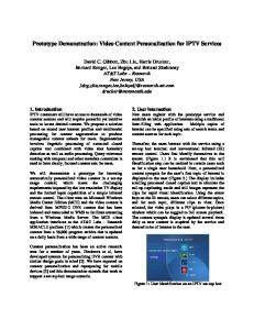
There is currently a huge effort in the experimental gravity wave world community to build detectors that will detect gravitational waves. There are six detectors that will come on line in the next 10 years. An array of detectors is important in order to correlate the data since the signal to noise ratio will not be very large. The United States project, LIGO, will be the one most frequently discussed in this work. It is a power-recycled Michelson with 4-km long arm cavities [25].
21 Sapphire test masses
−21
10
Shot noise Int. thermal Susp. thermal Radiation pressure Total noise
−22
h(f) / Hz1/2
10
−23
10
−24
10
−25
10
1
10
2
3
10
10 f / Hz
Figure 1.8: Expected noise levels for LIGO II The first generation of LIGO has been designed to give a strain sensitivity of ∼ 10−22 /Hz1/2 . The more favorable estimates of event rates that this detector will be able to sense is not better than a few per year, and most likely no events will be detectable. In order to guarantee that the detector will see gravitational radiation at a rate of better than one per year the sensitivity must be increased by at least a factor of 10. In order to do that all the noise sources mentioned previously must be improved upon. Figure (1.8) shows the expected noise in LIGO II for sapphire test masses [26]. Every noise source contributes significantly to the total noise curve. The most critical are internal thermal noise of the test masses themselves and the shot noise of the detector. The next generation of gravitational wave detectors will require all the techniques to reduce shot noise discussed in Section 1.2.1. In order for the detector to work a scheme for locking all the mirrors so that the light is resonant in the appropriate places needs to be devised. That is the main thrust of this work.
22 Chapter 2 will analyze the sensitivity of different interferometer configurations. A detailed transfer function for different configurations will be derived. Control schemes for the different configurations will be discussed and when possible, calculated. A method for comparing different control schemes for the same configuration will be presented. A detailed explanation for how the experimental dual-recycled tabletop instrument was controlled will be presented. The frequency response of a signal-recycled instrument will be discussed in more detail. Chapter 3 will discuss the prototype dual-recycled cavity-enhanced interferometer that was constructed on a tabletop. It will explain in detail how the parameters were decided on. It will give a detailed explanation for the error signals expected from the instrument. The instrument will be characterized through measurements of losses and the amount of power buildup in cavities. The performance of the error signals will be assessed with a measurement of the locking matrix. The low frequency sensitivity of the instrument will be shown. The measurement of the high frequency response of the dual-recycled and slightly detuned instrument will be presented and compared to the predictions. Chapter 4 will summarize the work done. It will draw some final conclusions. Possible future work will be discussed.
CHAPTER 2 THEORY The analysis and control of a complex interferometer requires some general theory along with detailed calculations. This chapter will discuss the input light field, the generation of additional frequency components on that light field and detection of the fields. It will then explain how those detected light fields can be used to control the interferometer. The next step will be a careful analysis of the different topologies for the instrument, including a section on the control signals for each topology. There are two regimes in which an optical configuration can be analyzed. The first is its response to time dependent perturbations. This analysis ignores the storage times of complex cavities, but it is very useful in developing a locking scheme for the interferometer. It will also explain the slow time response of the interferometer to gravitational radiation, where the signal frequency is much lower than the storage time of any of the cavities. The second regime is the response to time dependent perturbations. This frequency analysis is fundamental to how the interferometer will respond to the gravity wave in general. In order to understand how signals are generated in complicated multi-cavity interferometers, it is useful to build up a model for the static case using subsections. This will allow us eventually to express a full transfer function of the complete interferometer, which will depend on the frequency of the light. Although there are programs which allow modeling of different interferometer configurations [27], one needs to go through this exercise in order to develop and understand a locking scheme. The frequency analysis will be accomplished largely through the modeling program Finesse.
23
24 2.1
Light Fields
In most cases the light field going into a complex interferometer has some frequency shifted components. The advantages of this will be explored more thoroughly when we discuss locking the cavities and the Michelson interferometer to the center frequency, or carrier. The frequency shifted fields come in two flavors, either single sideband or paired sideband. Since our experiment uses only paired sidebands, that is the situation that we consider in detail. 2.1.1
Generating Sidebands
In order to generate a pair of sidebands the carrier passes through an electrooptic modulator (EOM) [28]. The modulator is driven with a sine wave typically in the RF frequency region which modulates the index of refraction through the electrooptic effect. This results in an effective path length change that oscillates at the drive frequency. The output field is then
Epm = E0 e−i(ω0 t+m sin Ωt) ,
(2.1)
where ω0 is the light frequency, and Ω is the frequency at which the EOM is driven. m is related to the amplitude of the driving frequency. If we assume m is much less than one, as would normally be the case, then Equation (2.1) becomes
Epm ' E0 e−iω0 t (1 − im sin Ωt) � � m m ' E0 e−iω0 t + e−i(ω0 +Ω)t − e−i(ω0 −Ω)t 2 2
(2.2) (2.3)
Figure (2.1) shows how the electric field looks in a frequency domain. There is a phase relationship between the carrier and the sidebands that changes with time.
25
E0
E1
E-1 Figure 2.1: Carrier with sidebands in frequency space The sidebands rotate in the complex plane in opposite directions with respect to the carrier at frequency Ω. For a good discussion of this, see Mizuno’s thesis [29, p.20-28]. At this point it is important to note that light reflecting off a mirror oscillating in the direction of the incident light z at a given frequency has the exact same effect on the light field. It takes some portion off the carrier and frequency shifts it, such that it creates a pair of sidebands. This is the same effect as doppler shifting. As the wavefronts reflect off a mirror moving opposite the direction of incidence, the reflected wave fronts are closer together than the original wavefronts, shifting the frequency up. As the light reflects off a mirror moving away from the incident light it shifts the reflected light’s frequency down. For a mirror moving sinusoidally the reflected light has the form of Equation (2.1) It follows that when a gravity wave interacts with an arm of the interferometer, given Equation (1.19), the effect the gravitational wave has on the light field in the instrument can be described as a pair of frequency shifted sidebands. This realization becomes very useful in synthesizing signals. Rather than trying to move a mirror to simulate a gravitational wave, light can be added to the system through the end
26 mirror of one of the arms. If the added light is offset from the carrier by a frequency ωg then it simulates one half of the pair of sidebands that would be created by the interaction of a gravitational wave of frequency ωg with the detector. 2.1.2
Sideband Detection
Once this field has traveled through an optical device, be it either a cavity or complex interferometer, the sideband amplitudes and phases have changed due to the frequency dependent transfer function, T (k). We can write an electric field with paired sidebands after it has interacted with an arbitrary transfer function as h i m m E = T (k0 ) + T (k+ ) e−iΩt − T (k− ) eiΩt E0 e−iωt 2 2
(2.4)
where k± = k0 ± kΩ , k = ωc , and E0 is the amplitude of the carrier before interacting with the system. A photodetector will only detect the power of the total field, or
P = EE ∗ ,
(2.5)
which leads to
EE ∗ =D.C. +
m {T (k0 ) T ∗ (k+ ) + T ∗ (k0 ) T (k+ ) 2
(2.6)
− T (k0 ) T ∗ (k− ) − T ∗ (k0 ) T (k− )} |E0 |2 cos Ωt +i
m {T (k0 ) T ∗ (k+ ) − T ∗ (k0 ) T (k+ ) 2
+ T (k0 ) T ∗ (k− ) − T ∗ (k0 ) T (k− )} |E0 |2 sin Ωt
(2.7)
27 Realizing that a + a∗ = 2< {a} and a − a∗ = 2= {a} allows us to write P =D.C. + m< {T (k0 ) [T (k+ ) − T (k− )]∗ } |E0 |2 cos Ωt
(2.8)
− m= {T (k0 ) [T (k+ ) + T (k− )]∗ } |E0 |2 sin Ωt
(2.9)
Taking the photocurrent and using heterodyne detection [30, p.885-902], the signal is beat against a sine wave with the appropriate demodulation phase, φ, such that Ω s= 2π
Z
2π Ω
P cos (Ωt + φ) dt.
(2.10)
0
Choosing the appropriate phase, φ, picks up a factor of
1 2
from the integration
and yields the final results of m = {T (k0 ) [T (k+ ) + T (k− )]∗ } |E0 |2 2 m = < {T (k0 ) [T (k+ ) − T (k0 )]∗ } |E0 |2 2
sinphase = − squadrature
(2.11) (2.12)
These two signals, the in-phase and the quadrature, can be generated by two different processes. The in-phase component will be generated when there is a phase shift between the sidebands and the carrier. Assuming that the sideband phase does not change as the system departs from its operating point, but that the carrier receives some phase shift, then it is the beat of the carrier with the sidebands acting as a local oscillator that would create a signal which gives information about how the system phase shifted the carrier. This signal could be used to control the system so that the phase shift imparted to the carrier does not change with time. This signal is known as an error signal. The in-phase signal will be the sine of the phase difference between the paired sidebands and the carrier, which is a good error signal since it is zero when
28 the phases are the same, and has opposite signs depending on whether the phase shift is positive or negative. A quadrature signal will be created when there is an imbalance in the paired sideband amplitudes. Assuming that the carrier and sideband phases do not change as the system departs from its operating point, but that the amplitude of the two sidebands changes antisymmetricly, then an error signal is created in this component. Again, the error signal is zero at the operating point and changes sign depending on which direction it has departed. There are other ways in which the error signals can be created. For example, a change in the phase of the sidebands will show up in the quadrature signal. Often the transfer function of the system acting on the input light field will create a signal that appears in both quadratures. If, for example, the transfer function depends on two degrees of freedom, it is desirable to have signals to sense these degrees of freedom that are independent from each other. The input light field and the free parameters in the transfer function are usually chosen such that the degree of freedom that creates the signal is as pure in one component as possible. This leaves the other component of the signal to be used for the other degree of freedom, and the two processes then create error signals that are independent from one another. There may be some confusion here as to why the in-phase signal is obtained when mixing down with sin Ωt and the quadrature signal is obtained when mixing down with cos Ωt. Typically the situation would be the reverse, since the sine is the imaginary part and the cosine the real part of the complex optical field. This should not be a concern since it depends on the phase used to demodulate the signal. If one started the derivation with sidebands being generated with a cosine modulation rather than the sine that was chosen here, then the final demodulation phases would have been shifted by π and you would have the standard concept of in-phase and
29 quadrature. The important thing to realize is that there are two signals that are orthogonal to each other. 2.2
Locking Matrix
Ultimately the goal of the interferometer is to obtain the highest sensitivity to the gravitational wave. To accomplish this, complex optical configurations are used with many degrees of freedom. These degrees of freedom must be sufficiently controlled such that they don’t introduce noise into the gravity-wave channel. Optimally a change of one of the degrees of freedom from the operating point would not affect the other degrees of freedom. However, that is usually not the case in complex optical configurations. Take the example of a power-recycled Michelson with arm cavities. A change in the length of the arm cavities results in a phase shift of the carrier coming from the arms. This phase shift causes the power-recycling cavity to no longer have a buildup inside it, since the incoming light is no longer perfectly constructively interfering with the light in the cavity. The power recycling factor is reduced, thus reducing the sensitivity to the gravitational wave signal.
DL
+
M
G Figure 2.2: Feedback loop for a general system
S
30 There is a general way to discuss how independent the signals used to control the degrees of freedom are and how to decide on a control scheme. Figure 2.2 shows a general system with feedback. The matrix M is the optical system, and in general not diagonal. The matrix G is the gain matrix, and for simplicity sake is usually → − diagonal. The vector S are the error signals that we use to feed back to the degrees −→ of freedom. The vector ∆L is the disturbance of each of the degrees of freedom. We can now write down the error signals in general as − → −→ → − S = M∆L + G M S .
(2.13)
Solving this equation for the signal vector we get − → S =
−→ M ∆L. 1−GM
(2.14)
−→ The situation that requires analysis is two degrees of freedom, where ∆L = {∆L1 , ∆L2 } and M is a 2 by 2 matrix. We will use this as a basic building block for much more complicated situations. In this case G1 0 G= 0 G 2
(2.15)
The locking matrix is created from the equations that govern how S1 and S2 depend on the degrees of freedom. Writing down the error signals as ∂S1 ∆L1 + ∂L1 ∂S2 S2 = ∆L1 + ∂L1
S1 =
∂S1 ∆L2 ∂L2 ∂S2 ∆L2 ∂L2
(2.16) (2.17)
31 The locking matrix is the Jacobian, defined as ∂S1 ∂L1 M = ∂S2 ∂L1
∂S1 ∂L2
∂S2 ∂L2
(2.18)
It is now useful to solve for the two signals in order to see how one signal depends on the two degrees of freedom. After some linear algebra the results are � S1 =
S2 =
−G2 det M +
∂S1 ∂L1
�
∆L1 +
∂S1 ∆L2 ∂L2
∂S1 ∂S2 1 − ∂L G1 − ∂L G2 − G1 G2 det M 1 2 � � ∂S2 ∂S2 −G1 det M + ∂L ∆L2 + ∂L ∆L1 2 1
1−
∂S1 G ∂L1 1
−
∂S2 G ∂L2 2
− G1 G2 det M
(2.19)
.
(2.20)
There are a few cases to consider. The first case is when the two degrees of freedom truly are independent from each other. That is equivalent to assuming that M is diagonal. We can also assume
∂S1,2 G ∂L1,2 1,2
� 1 for the steady state solution, since
we want enough feedback to hold the resonant conditions for the light. Then these equations become
S1 =
S2 =
1
1
∂S1 ∂L1 ∆L1 ∂S1 − ∂L G 1 1
'−
∆L1 G1
(2.21)
∂S2 ∂L2 ∆L2 ∂S2 − ∂L G 2 2
'−
∆L2 G2
(2.22)
The second case to consider is when the off-diagonal terms in M start to get large compared to the diagonal terms. In this case the signals start to get mixed. Without taking special steps with the gain distributions, changes in one degree of freedom appear in the error signal for the other degree of freedom causing the system
32 to try to compensate for this signal. This is a bad situation, and in general we want Si to be dependent only on ∆Li Taking Equation (2.20), we realize that for S2 to be dominated by ∆L2 then the condition G1 det M −
∂S2 ∂S2 � ∂L2 ∂L1
(2.23)
must be true. Investigating the case where the degree of freedom L1 dominates signal S2 , then ∂S2 ∂L1
�
∂S2 . ∂L2
We can now write a simple expression for G1 .
G1 �
∂S2 ∂L1
G1 � ∂S2 ∂L1
If
∂S2 ∂L2 ∂S2 ∂L1
=
∂S1 ∂L2 ∂S1 ∂L1
(2.24)
det M 1 � ∂S2 ∂L2 ∂S2 ∂L1
−
∂S1 ∂L2 ∂S1 ∂L1
�
(2.25)
, corresponding to the det M = 0, the signals are linearly dependent.
We cannot lock this system since there is no unique locking point. As long as the system is not very linearly dependent, the gain does not need to be abnormally high. As the system becomes more and more linearly dependent, then det M → 0 and in order to achieve lock G1 → ∞. There is an absolute measure for how orthogonal the signals are to one another, given by the cross product of the two signals. The angle between the two signals is defined as
− → → − S1 × S2 sin α ≡ − → − → S1 S2
(2.26)
33 Looking at equations (2.16) and (2.17) we can see that the cross product of the two signals is ∂S1 ∂S2 ∂S1 ∂S2 ∂L1 ∂L2 − ∂L 2 ∂L1 q sin α = q , ∂S1 ∂S1 ∂S2 ∂S2 + + ∂L1 ∂L2 ∂L1 ∂L2
(2.27)
which we recognize as
sin α = q
∂S1 ∂L1
+
det M q
∂S1 ∂L2
∂S2 ∂L1
. +
(2.28)
∂S2 ∂L2
The smaller α is, the more linearly dependent the two signals are. This gives us an absolute measure with which to compare locking schemes. 2.3
Simple Cavity
The simple cavity is the most fundamental improvement for an interferometric gravitational wave detector. It is very useful to explore the properties of a simple cavity completely. Since a suspended cavity cannot detect gravitational radiation the frequency analysis will be saved for when it is applicable in a detector.
r2, t2
Einb
Etrans +
-
L
Eino
r1, t1
-
+
Erefl E0
Figure 2.3: Fields in a simple cavity
2.3.1
Light Fields
Figure (2.3) shows the notation used. We adopt a few conventions here that are not necessarily universal. Light reflected off the coated side of a mirror gets a minus sign. Light reflected off the substrate side of the mirror gets a plus sign.
34 All transmitted light is real and positive and the substrates have zero thickness. As for notation, all fields traveling away from a mirror have the subscript o and all fields traveling to the mirror have the subscript b. The mirror reflectivities and transmissivities, ri and ti , are for field amplitudes. For power quantities they are related by Ri = |ri |2 and Ti = |ti |2 . Writing all the equations for the fields gives
Eino = t1 E0 − r1 Einb
(2.29)
Einb = −r2 e−2ikL Eino
(2.30)
Etrans = t2 e−ikL Eino Eref l = r1 E0 + t1 Einb .
(2.31) (2.32)
Continuing on in painful detail, we substitute Equation (2.29) into Equation (2.30) and solve for Einb :
Einb
Einb = −r2 e−2ikL (t1 E0 − r1 Einb ) � 1 − r1 r2 e−2ikL = −r2 t1 e−2ikL E0 Einb =
−r2 t1 e−2ikL E0 1 − r1 r2 e−2ikL
(2.33) (2.34) (2.35)
Solving for the other fields gives : t1 E0 1 − r1 r2 e−2ikL t1 t2 e−ikL = E0 1 − r1 r2 e−2ikL r1 − r2 (r12 + t21 ) e−2ikL = E0 . 1 − r1 r2 e−2ikL
Eino = Etrans Eref l
(2.36) (2.37) (2.38)
35 It is useful to define a complex reflectivity of the cavity such that
Eref l = −rF P E0 .
(2.39)
Assuming that there are no losses in the coating (generally a good assumption), so that r12 + t21 = 1, we can write
rF P =
−r1 + r2 e−2ikL . 1 − r1 r2 e−2ikL
(2.40)
There is a lot to be learned from these equations. If we assume that the cavities are resonant for the carrier, such that L =
nλ , 2
we can define the buildup inside the
cavity as Eino 1 = ≥ 1. t1 E0 1 − r1 r 2
(2.41)
This number is always greater than or equal to 1 since the limit where r2 → 0 implies that the field inside is simply the light transmitted through the first mirror. As r2 gets larger than 0 the amplitude of electric field in the cavity increases. This changes if the light is not on resonance. The light reflected from the cavity is Eref l r1 − r 2 = . E0 1 − r 1 r2
(2.42)
The numerator is negative if r2 > r1 , and reflected light is shifted by 180 degrees in phase from the incoming light. This condition is known as an over-coupled cavity. If r2 < r1 then the reflected light has the same phase as the incoming light, which is known as an under-coupled cavity. If r2 = r1 , then there is no light reflected from the cavity, and it is impedance matched, or critically coupled. If there are no losses, then the transmitted power of the impedance matched cavity is equal to the input power. Losses in the cavity can often be combined to be included into the r2 term,
36 such that r2 → r2
p
1 − s2loss and t2 is unchanged. This approximation concentrates
all the losses in the second mirror, and does not affect any of the equations used thus far. It is also useful to calculate the phase shift that the light receives from a cavity. From Equation (2.42) we calculate
tan ϕ =
r1 (1 + R2 ) − r2 (1 + R1 ) cos (2kL) r2 (1 − R1 ) sin (2kL)
(2.43)
Figure 2.4 shows the phase shift that the reflected light receives from an overcoupled cavity. When the light is resonant with the cavity the reflected light is shifted by 180 degrees. When the light is antiresonant the phase shift is zero or 2π. This will be a useful fact for deciding where to place sidebands with respect to a cavity’s free spectral range in order to get the most useful locking signals.
π
π
π
Figure 2.4: Phase shift of light reflected from an over-coupled cavity There are two quantities that are often used to define a cavity. They are related to the length of the cavity and the reflectivities of the mirrors. The free spectral
37
− 2
Figure 2.5: Transmission of an impedance matched cavity range of a cavity is defined as FSR =
c . 2L
(2.44)
Changing the cavity’s length on the order of wavelengths causes the cavity to go through resonances every free spectral range. The resonances occur at a length change equal to a half wavelength of the input light. If there are sidebands on the light, and they are at a frequency that equals the FSR then they will also be resonant in the cavity when the carrier is resonant. The finesse of the cavity is defined as √ π r 1 r2 F = . 1 − r1 r2
(2.45)
This quantity is a measure of how much light is built up in the cavity. Figure (2.5) shows the transmitted field of a cavity as it is scanned over a wavelength. The physical parameters that can be measured are the FSR and the full
38 width half maximum (FWHM). The FWHM is related to the Finesse and the FSR [31, p.408-436] by
FWHM ≈
FSR . F
(2.46)
One can determine the reflectivities of the mirrors of a cavity by measuring the FWHM, the FSR, and the losses of the cavity. By measuring the FWHM and the FSR the finesse can be calculated from Equation (2.46). Solving Equation (2.45) for the square root of the reflectivities gives
A≡
√
r 1 r2 =
−π ±
√
π 2 + 4F 2 2F
(2.47)
and A2 . r1
(2.48)
|Eref l | = sloss |E0 | ,
(2.49)
r2 =
Defining the amplitude loss as
we can write Equation (2.42) as r sloss =
2
r1 − Ar1 Pref l = P0 1 − A2
(2.50)
and solving for r1 gives q sloss (1 − A ) ± (sloss )2 (1 − A2 )2 + 4A2 2
r1 =
2
.
(2.51)
39 Note that s2loss is a direct measurement of the total power loss in the cavity. This is accomplished by measuring the power reflected from the cavity on resonance and dividing it by the power reflected when the cavity is off-resonant. Losses in a cavity are rarely negligible. Assuming 1/8th of a percent losses on each bounce off a mirror, which seems to be pretty realistic for the mirrors in this experiment, a cavity with a finesse of 60 has total losses of almost 10%. If the light isn’t on resonance then the analysis needs to be redone. This will be useful to calculate the length of a cavity when the RF sideband is sitting somewhere near the FWHM of the cavity. We can calculate the length of the detuning from the measurement of the power buildup inside the cavity. 2 |Eino |2 1 ≡B = T1 |E0 |2 1 − r1 r2 e−2ikL
(2.52)
gives
cos (2kL) =
1 + R1 R2 − 2r1 r2
1 B
(2.53)
Here we’ve used the familiar ri2 = Ri . In order to calculate the effective reflectivity of the end mirror we need to use the reflected field. We’ll divide the incoming field by the reflectivity of the first mirror, since normally the fields measured from a cavity are the reflected field when the cavity is locked, and the reflected field when a beam block as been inserted into the cavity. Solving these equations |Eref l |2 |E0 |2 R1
1 = R1
r1 − r2 e−2ikL 2 1 − r1 r2 e−2ikL ≡ C,
2 C 1 = r1 − r2 e−2ikL , B R1
(2.54) (2.55)
40 gives � C 1 + R1 B −1 − R2 = 1 − R1
1 B
.
(2.56)
It will be useful to calculate the reflectivity of a cavity for small changes in length. This will not only be used for calculating how the gravity-wave signal shows up in the light fields of the cavity, but also will be used to generate error signals for the cavity. For a change in length of the cavity L → L ± δl, Equation (2.40) can be written as
rF P =
−r1 + r2 e−2ik(L±δl) . 1 − r1 r2 e−2ik(L±δl)
(2.57)
Assuming that the arm cavity is on resonance for the light, Equation (2.57) becomes
rF P =
2.3.2
−r1 + r2 e−2ik(±δl) . 1 − r1 r2 e−2ik(±δl)
(2.58)
Error Signals
There are two common processes that generate an error signal [12]. We showed that signals can be generated either by the change of the phase of the carrier with respect to the sidebands, resulting in an in-phase signal, or by an amplitude difference in the paired sidebands, resulting in a quadrature signal. An in-phase signal is created when the carrier receives a phase shift relative to the sidebands from a slight change in length of the cavity, but the amplitudes of the sidebands stay that same. The obvious place to put the sidebands would be at the antiresonant points of the cavity, which is half the free spectral range. At that point the sidebands are very insensitive to length changes of the cavity. Figure 2.6 shows
41
Figure 2.6: Light fields with antiresonant sidebands in a cavity where the electric fields lie with respect to the cavity resonances in frequency space. From figure 2.4 we can see that the sidebands do not receive any phase shift when they are placed at half the free spectral range. Referring to Equation (2.38) and using the fact that the sidebands are antiresonant, we can write the reflected sideband fields as
E±1 ref l =
r1 + r2 E±1 input 1 + r 1 r2
(2.59)
The electric fields reflected off the cavity can now be expressed as � r1 − r2 e−2ik0 δl m r1 + r2 −iΩt m r1 + r2 iΩt E= + e − e E0 e−2iω0 t −2ik δl 0 1 − r1 r 2 e 2 1 + r 1 r2 2 1 + r1 r2 �
(2.60)
Comparing this field to equations (2.11) and (2.12), we can calculate the error signal. Since the sideband transfer function amplitudes are equal, as expected, then
42 the quadrature component is zero. The sideband transfer functions are also real as written, and so we just need to calculate the imaginary part of the reflected carrier.
� � r1 − r2 e−2ik0 δl 1 − r1 r2 e2ik0 δl = {E0 ref l } = 1 + R1 R2 − 2r1 r2 cos (2k0 δl) r2 (1 − R1 ) sin (2k0 δl) = 1 + R1 R2 − 2r1 r2 cos (2k0 δl) =
�
(2.61) (2.62)
Putting this into Equation (2.11) gives
sinphase = −m
r 1 + r2 r2 (1 − R1 ) sin 2k0 δl . 1 + r1 r2 1 + R1 R2 − 2r1 r2 cos 2k0 δl
(2.63)
In hindsight, the general shape of Equation (2.63) would have been easy to guess. The carrier picks up an extra phase shift from movement of the back mirror of the cavity that the sideband doesn’t see since it is reflected directly off the front mirror. The phase shift would be 2k0 δl. Equation (2.11) shows that the overall error signal would go like the sine of the phase shift. Since that equation also says that the amplitude of the error signal corresponds to the amplitude of the carrier, we would also predict the denominator. The amplitudes of the sidebands are also what would be expected. Figure (2.7) shows what the in-phase error signal looks like when the sidebands have been placed at the antiresonances of the cavity. The slope at the center of the error signal is related to the finesse of the cavity. The features at half the free spectral range is the signal created by the sidebands becoming resonant in the cavity. The locking range of the signal is defined as when the signal changes sign. In this case the locking range is λ/4. For more complicated systems the locking range can become small, and it is then a concern since the system must be very close to the operating point in order to generate the correct locking signal.
43
−λ
λ
Figure 2.7: In-phase error signal for a cavity in reflection The quadrature error signal can not be produced without also producing the in-phase signal. There is no frequency for the sidebands such that a change in length of the cavity results in a change of amplitude of the sidebands but not the phase of the sidebands relative to the carrier. An important point here is the concept of a local oscillator. For the two error signal quadratures, the carrier and the sidebands shift in their role of local oscillator. In the case where a signal is produced by a phase shift of the carrier, the sidebands are the local oscillator, providing a constant phase reference. There must be sideband present in order to detect an error signal. In the case where the error signal is created by an imbalance in the amplitudes of the sidebands the carrier is playing the role of the local oscillator. This means that if a cavity is impedance matched for the carrier, then there is an in-phase locking signal in reflection, but there is no quadrature signal. If one can take the signal from inside the cavity, then both error signals are present.
44 2.4
Michelson
The simple Michelson is the fundamental building block for a gravitational wave detector. The Michelson’s control is important to investigate in order to understand how to accomplish that control in a more complicated configuration. The frequency response is a simple cosine function as would be expected in any Michelson, and does not deserve any special attention.
+ -
rp, tp
dl
lp Epo
ri, ti
+
Epb
Eib -
dl
li
Erefl
Eio
+
-
rbs, tbs
E0
Eantisym Figure 2.8: Fields in a simple Michelson
2.4.1
Light Fields
The sensitivity of a simple Michelson to a differential change in the arm lengths is a relatively easy calculation. A few conventions need to be chosen. As in the case of the simple cavity all reflectivities and transmissivities of simple mirrors are real and positive. Light reflected off the coated side of the optic in air will get a minus
45 sign, light reflected off the coated side in the substrate will have a plus sign. This applies to the beam splitter as well. Figure (2.8) shows the notation that will be used. The fields are all drawn as they interact with the beam splitter. A quick explanation of the subscripts is useful. Fields and optics in the arm that are in line with the incoming beam get a subscript i. Fields and optics that are perpendicular get a subscript p. Fields traveling away from the optic get a subscript o and fields traveling back toward the optic get a subscript b.
Eio = tbs E0
(2.64)
Eib = −ri e−2ikli Eio = −ri tbs e−2ikli E0
(2.65)
Epo = −rbs E0
(2.66)
Epb = −rp e−2iklp Epo = rp rbs e−2iklp E0
(2.67)
These equations give us a solution for the transfer function of the light to the antisymmetric port:
Eantisym = rbs Eib + tbs Epb � T (k)antisym = rbs tbs rp e−2iklp − ri e−2ikli � � l +l l −l l −l −2ik p 2 i −2ik p 2 i 2ik p 2 i = rbs tbs e rp e − ri e . ≡ tM I (k)
(2.68) (2.69) (2.70) (2.71)
46 If we assume that the lengths of the two arms are unchanged except for a small differential movement such that
lp = lp − δl
li = li + δl,
(2.72)
and that the end mirrors have the same reflectivity, r2 then (2.70) becomes
T (k)antisym
� � �� lp +li lp − li − δl e−2ik 2 . = 2irbs tbs r2 sin 2k 2
(2.73)
We can see that the choice of how we define reflections and transmissions at surfaces has created an antisymmetric port that is dark for equal length arms. It is also useful to write down the transfer function for the reflected port � � l −l lp −li lp +li 2 −2ik p 2 i T (k)ref l = − rp rbs e + ri t2bs e2ik 2 e−2ik 2 ≡ −rM I (k) .
2.4.2
(2.74) (2.75)
Error Signals
We have already derived the transfer functions of the Michelson interferometer. It makes sense to lock the Michelson at the antisymmetric port using an in-phase signal. In order to do this we need to set the sideband at
Ω=
RESM I 2
(2.76)
c . 2 (lp − li )
(2.77)
where
RESM I =
This ensures that the sidebands are bright in the antisymmetric port.
47
+
−
−λ
λ
Figure 2.9: Transfer function of the Michelson Figure (2.9) shows where the fields lie with respect to the carrier. The two sidebands in fact do have the same sign at the antisymmetric port. This is the result of having opposite signs at the input of the Michelson, and the fact that the transfer function of the Michelson to the antisymmetric port flips the sign of the upper sideband, but not the lower sideband, as is clear from the figure. The carrier has a sign opposite that of the sidebands. It is useful to solve this situation analytically. Writing down the field for the carrier at the antisymmetric port using a 50/50 beam splitter and full reflector end mirrors we get E0 antisym = i sin (2k0 δl) e−2ik0
lp +li 2
E0
(2.78)
The sidebands take a little more work to get. From Equation (2.70) we get
−2ik±
E±1 = −ie
lp +li 2
�
lp − li sin 2k± 2
� (2.79)
48 Substituting lp = lp − δl, li = li + δl and realizing that setting the carrier to be dark i at this port, and the sidebands to be bright gives the conditions 2k0 lp −l = nπ and 2 i 2k± lp −l = (n + 1) π2 yields 2
E± = ∓ie−2ik±
lp +li 2
cos 2k± δl.
(2.80)
Writing
cos 2 (k0 ± kΩ ) δl = cos (2k0 δl) cos (2kΩ δl) ∓ sin (2k0 δl) sin (2kΩ δl) ,
(2.81)
and taking δl