Denoising and Feature Extraction Algorithms Using ...

SS symmetry Article

Denoising and Feature Extraction Algorithms Using NPE Combined with VMD and Their Applications in Ship-Radiated Noise Yuxing Li *

ID

, Yaan Li *, Xiao Chen and Jing Yu

ID

School of Marine Science and Technology, Northwestern Polytechnical University, Xi’an 710072, China; [email protected] (X.C.); [email protected] (J.Y.) * Correspondence: [email protected] (Yu.L.); [email protected] (Ya.L.); Tel.: +86-29-8849-5817 (Ya.L.) Received: 10 October 2017; Accepted: 27 October 2017; Published: 1 November 2017

Abstract: A new denoising algorithm and feature extraction algorithm that combine a new kind of permutation entropy (NPE) and variational mode decomposition (VMD) are put forward in this paper. VMD is a new self-adaptive signal processing algorithm, which is more robust to sampling and noise, and also can overcome the problem of mode mixing in empirical mode decomposition (EMD) and ensemble EMD (EEMD). Permutation entropy (PE), as a nonlinear dynamics parameter, is a powerful tool that can describe the complexity of a time series. NPE, a new version of PE, is interpreted as distance to white noise, which shows a reverse trend to PE and has better stability than PE. In this paper, three kinds of ship-radiated noise (SN) signal are decomposed by VMD algorithm, and a series of intrinsic mode functions (IMF) are obtained. The NPEs of all the IMFs are calculated, the noise IMFs are screened out according to the value of NPE, and the process of denoising can be realized by reconstructing the rest of IMFs. Then the reconstructed SN signal is decomposed by VMD algorithm again, and one IMF containing the most dominant information is chosen to represent the original SN signal. Finally, NPE of the chosen IMF is calculated as a new complexity feature, which constitutes the input of the support vector machine (SVM) for pattern recognition of SN. Compared with the existing denoising algorithms and feature extraction algorithms, the effectiveness of proposed algorithms is validated using the numerical simulation signal and the different kinds of SN signal. Keywords: denoising; feature extraction; VMD; permutation entropy; ship-radiated noise; pattern recognition

1. Introduction As a part of underwater acoustic signal processing, research on denoising and feature extraction of ship play a very important role in the modern sea battlefield. SN signal contains more characteristic parameters of ship, which is an important indicator of the performance of ship. Therefore, the denoising and feature extraction for SN are critical technologies in the underwater acoustic field [1]. Due to the presence of noise, the physical characteristics of real signal are covered up. That has a great influence on signal analysis, detection, feature extraction, classification and recognition. As the premise of feature extraction, denoising can improve the performance of feature extraction for SN. Research on feature extraction for SN is helpful for the accurate identification of enemy targets, and has significance in theory and practice [2]. Because underwater acoustic signal is non-stationary, non-Gaussian and nonlinear, the traditional signal processing algorithms cannot process it effectively. The Fourier Transform can only show characteristics in the frequency domain; also, the wavelet transform has the limits of the selection of basic functions and decomposition level. As a completely self-adaptive signal processing algorithm, Symmetry 2017, 9, 256; doi:10.3390/sym9110256

www.mdpi.com/journal/symmetry

Symmetry 2017, 9, 256

2 of 18

EMD is widely applied not only to fault diagnosis and medical science but also in underwater acoustic signal processing and economics [3]. EMD can decompose the multi-component signal into a series of IMFs based on the local characteristics; nevertheless, EMD has the problems of mode mixing and end effects. To solve the problem of mode mixing, an improved algorithm called EEMD was proposed by Wu et al. in 2009 [4], which can effectively reduce the degree of mode mixing by adding white noise repeatedly. However, both EMD and EEMD lack the foundation of mathematical theory and have the defect of poor robustness [5]. VMD [6], first introduced by Dragomiretskiy et al., is a non-recursive algorithm to analyze non-linear and non-stationary signal, which can adaptively decompose a complex signal into a series of quasi-orthogonal IMFs [7]. Each IMF is compact around a center frequency which can be estimated online. Compared with the EMD and EEMD algorithms, VMD has not only a solid theoretical foundation but also good robustness to noise. It has been applied in the fields of biomedical sciences [8,9], mechanical diagnosis [10] and underwater acoustic signal processing [11]. PE is one of the most effective ways to detect the randomness and dynamic changes of time sequence based on comparison of neighboring values [12–14]. However, NPE [15], a new kind of PE, was proposed to classify different sleep stages by Bandt in 2017. NPE is interpreted as distance to white noise, and is regarded as a key parameter that measures depth of sleep. Compared with PE, NPE shows a reverse trend to PE and has better stability for different lengths of time series. There is a class of denoising algorithms to eliminate noise, which include signal decomposition, screening and reconstruction of components. The basic idea of these algorithms extracts components of signal that was obtained by means of a signal decomposition algorithm and identifies and removes noise components according to the screening principle. Then, the useful components of signal are reconstructed to realize denoising. It is important to select appropriate decomposition algorithm and screening criteria. For example, the denoising algorithm using wavelet analysis has been widely used in different kinds of fields, and achieved good results [16,17]. However, it is limited by the selection of wavelet basis function and the decomposition level [18]. In addition, denoising algorithms based on EMD and its extended algorithms have been extensively studied. In research [19], the high-frequency IMF obtained by EMD is regarded as a noise component, and the rest of the IMFs are reconstructed to achieve denoising. However, this algorithm cannot completely remove noise signal, and lead to the lack of some detailed information. To overcome the shortcomings of these denoising algorithms, some improved denoising algorithms are proposed, which mainly achieve denoising through threshold denoising for IMFs [20,21]. However, the selection of different threshold has a great impact on the result of denoising. These improved denoising algorithms still have some limitations. A new denoising algorithm based on VMD and correlation coefficient is proposed in [22]; it uses the IMFs obtained by VMD to reconstruct the IMFs according to the correlation coefficients between IMFs and original signal to realize denoising. However, the selection of correlation coefficient threshold is a difficult problem. Recently, many new feature extraction algorithms have been developed and are based on signal decomposition algorithms and measuring complexity in different fields [23–26]. In research [27], a novel fault feature extraction algorithm for rotating equipment is proposed using improved autoregressive minimum entropy deconvolution and VMD, which is proven to be a more powerful algorithm than the existing ones. In research [28], a feature extraction algorithm for partial discharge is proposed using sample entropy combined with VMD. In the field of underwater acoustic signal processing, PE and multi-scale PE (MPE), as complexity features, are used to extract complexity features of SN combined with EMD and VMD respectively in [11,29]. It has been verified that the two feature extraction algorithms outperform the traditional feature extraction algorithms [30,31]. In this paper, VMD algorithm is used to decompose simulation and real signals, which can accurately decompose signal into IMFs. In addition, NPE has a strong ability for noise recognition. Considering the better performance of VMD and NPE for SN signal, a new denoising algorithm and feature extraction algorithm are presented. The remainder of the paper is organized as follows: in Section 2, the algorithms of VMD, PE, and NPE are described; the review of the denoising and

Symmetry 2017, 9, 256

3 of 18

feature extraction algorithm is presented in Section 3; then, the denoising algorithm and feature extraction algorithm are, respectively, applied to SN signal in Sections 4 and 5; finally, Section 6 concludes this paper. 2. Theory Description 2.1. VMD Algorithm VMD, as a new signal processing algorithm, is able to adaptively decompose a multi-component signal into multiple numbers of quasi-orthogonal IMFs concurrently. By comparing with EMD and EEMD, VMD has a solid mathematical foundation and defined the IMF as amplitude-modulated-frequency-modulated (AM-FM) signal, like uk (t) = Ak (t) cos(φk (t)),

(1)

where t and Ak (t) represent time the envelope, φk (t) and uk (t) denote the phase and the IMFs. Each IMF has a center frequency and limited bandwidth. In the VMD algorithm, the key decomposition process is the constrained variational problem, which is expressed as  

min ∑ ∂t[(δ(t) + { u k },{ w k }  k =1 K

2 

 j − jwkt ) ∗ u ( t )] e

k πt



(2)

2

K

s.t. ∑ uk = s, k =1

where s represent the processed signal, K is the number of IMFs, ∗ represents convolution. δ and j stand for impulse response and imaginary unit. wk is the center frequency for each decomposed component, uk is also the decomposed mono-component. The above constrained variational problem in Equation (2) is addressed by using the penalty factor and the Lagrangian multiplier. The augmented Lagrangian is given by

L({uk }, {wk }, λ)

2

j = α ∑ ∂t[(δ(t) + πt ) ∗ uk (t)]e− jwkt

k =1 2

2

K K

+ f ( t ) − ∑ u k ( t ) + λ ( t ), f ( t ) − ∑ u k ( t ) ,

k =1 k =1 K

(3)

2

where λ and α are the Lagrangian multiplier and balancing parameter. The alternating direction multiplier method (ADMM) is applied to obtain the saddle point, then the uk , wk and λ are updated in frequency, like λˆ n (w) fˆ(w) − ∑ uˆ n (w) − ∑ uˆ n (w) + i k

2

1 + 2α(w − wkn )2 r ∞ n+1 2 dw 0 w uˆ k , = r 2 ∞ n +1 ˆ u dw 0 k

! ˆλn+1 (w) = λˆ n (w) + τ fˆ(w) − ∑ uˆ nn+1 (w) , k

,

(4)

(5)

(6)

Symmetry 2017, 9, 256 Symmetry 2017, 9, 256

4 of 18 4 of 17

τ indicate ∧ and where Fourier Transform and The timealgorithm step. Theexecutes algorithm until the where ∧ and τ indicate Fourier Transform and time step. untilexecutes the convergence convergence stop condition satisfied. The is stop condition is given by stop condition is satisfied. Theisstop condition given by

uˆ

ˆ 2

/ uˆ

2 < e，

n+1 −nu

uˆ k − uˆ k / uˆ nk < e, ∑k k

n +1 k

n 2 k 2

n 2 k 2

2

2

(7) (7)

where e is the accuracy for convergence. The process of algorithm is depicted in Figure 1. The where e is the accuracy for convergence. The process of algorithm is depicted in Figure 1. The detail of detail of VMD algorithm and experiment are shown in [6]. In this paper, the decomposition level VMD algorithm and experiment are shown in [6]. In this paper, the decomposition level K is the most K is the most important parameter, which can be set according to the decomposition level of EMD, important parameter, which can be set according to the decomposition level of EMD, and the penalty and the penalty factor is 2000. factor is 2000.

uˆ1k , w1k , λˆ1 , n = 0

n +1 uˆk wk

λˆ

Figure 1. 1. The flowchart of of VMD algorithm. Figure The flowchart VMD algorithm.

2.2. PEPE and NPE 2.2. and NPE PEPE was described toto detect the dynamic changes ofof time series byby comparison with neighboring was described detect the dynamic changes time series comparison with neighboring value of time series. Given a time series X = x , x , · · · , x with length N, the specific steps of PEof { } 2 N 1 value of time series. Given a time series X = x1 , x2 , , xN with length N, the specific steps are illustrated as follows: PE are illustrated as follows: (1) Embedded dimension m of the time series X with a time delay τ is constructed as follows: (1) Embedded dimension m of the time series X with a time delay τ is constructed as follows:   { x (1), x (1 + τ ), · · · , x (1 + (m − 1) τ )}    ..     { x.(1), x(1 + τ ), , x(1 + ( m − 1) τ )} , (8) {x ( j), x ( j + τ ), · · · , x ( j + (m − 1)τ )}   .     ..   , x( j ) , x( j + τ ), , x( j + (m − 1)τ )} (8)   { {x (K ), x (K + τ ), · · · , x (K + (m − 1)τ )} j = 1, 2, · · · , K

{

}

  where K is n − (m −  1)τ. j = 1, 2, , K { x ( K ), x( K + τ ), , x( K + (m − 1)τ )} (2) Each vector x (i ), x (i + τ ), · · · , x (i + (m − 1)τ )} of X is rearranged in ascending order as {

n −x((mi +− 1) ( j1τ−. 1)τ ) ≤ x (i + ( j2 − 1)τ ) ≤ · · · ≤ x (i + ( jm − 1)τ ). (9) (2) Each vector { x(i ), x(i + τ ),, x(i + (m − 1)τ )} of X is rearranged in ascending order as

where

K

is

If x (i + ( j1 − 1)τ ) = x (i + ( j2 − 1)τ ), then x (i + ( j1 − 1)τ ) ≤ x (i + ( j2 − 1)τ ) ( j1 ≤ j2 ).

Symmetry 2017, 9, 256

5 of 18

(3) Therefore, for time series X, each vector of X can be obtained as S(l ) = ( j1 , j2 , · · · , jm ),

(10)

where l = 1, 2, · · · , K, K ≤ m!. There are m! different symbol series, and S(l ) only indicates one symbol series. (4) The probability of each symbol series is calculated as P1 , P2 , · · · , PK , the PE of time series X can be defined according to the form of Shannon entropy as K

HP (m) = − ∑ Pj ln Pj .

(11)

j =1

(5) When Pj = 1/m!, H p (m) reaches the maximum ln(m!). Consequently, the PE can be standardized as HP = HP (m)/ ln(m!). (12) It is obvious that the value of H p is from 0 to 1. The details of PE method are shown in [12]. NPE, a new version of PE, is interpreted as distance to white noise. The steps of NPE is same with PE from step (1) to step (3). In step (4), the NPE of time series X can be defined as K

NH p =

1

∑ ( Pj − m! )

K

2

=

j =1

1

∑ Pj2 − m! ,

(13)

j =1

1 1 in the Formula (10), − Pj ln Pj is replaced by Pj2 , and a constant − m! is added. When Pj = m! , NHP reaches the smallest value 0, this means that the distance to white noise is 0. In order to prove the stability of NPE with different data lengths, simulation experiments of sinusoidal signal with different frequencies are carried out. The simulation signal is sin(2π f t), f represents frequency and sampling frequency is 104 Hz. For PE and NPE, the parameters of time delay and the embedded dimension are set as one and three respectively. Tables 1 and 2 show the PEs and NPEs of simulation signal with different frequencies and lengths, respectively. As it can be seen in Tables 1 and 2, NPE is more stable than PE for simulation signal with different frequencies and lengths.

Table 1. The PEs of different frequencies and data lengths. Data Length

100 Hz

200 Hz

500 Hz

1000 Hz

1000 2000 3000

0.445 0.4447 0.449

0.4869 0.4866 0.496

0.5937 0.5929 0.5834

0.7154 0.7139 0.6915

Table 2. The NPEs of different frequencies and data lengths. Data Length

100 Hz

200 Hz

500 Hz

1000 Hz

1000 2000 3000

0.3137 0.3137 0.3136

0.2948 0.2948 0.2945

0.2418 0.2419 0.2426

0.1678 0.1681 0.171

Table 2. The NPEs of different frequencies and data lengths.

Data Length

100 Hz

200 Hz

500 Hz

1000 Hz

1000 2000 3000

0.3137 0.3137 0.3136

0.2948 0.2948 0.2945

0.2418 0.2419 0.2426

0.1678 0.1681 0.171

Symmetry 2017, 9, 256

6 of 18

2.3. Analysis of the Simulation Signal Using VMD and NPE 2.3. Analysis of the Simulation Signal Using VMD and NPE In order to verify the effectiveness of the new algorithm, simulation experiments are carried out. In order tosignals verify are thegiven effectiveness of the new algorithm, simulation experiments are carried The simulation by out. The simulation signals are given by   cos(100πt 1 ==cos(100 π t) )   SS1   S2 = cos(200πt)  S 2 = cos(200π t ) , (14) (14)  S3 = cos(400πt，  )  S 3 = cos(400 π t )   + S2 + S3  SS ==S1S1 + S 2 + S3

-5

imf1

S

0

2 0 -2

imf2

5

2 0 -2

imf3

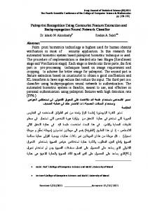
where S1, S3 areS 3theare three of S, sampling 104 Hz. The of 104 Hz. The , Sand thecomponents three components of S ,frequency sampling isfrequency is parameters S1 S2 2 and time delay and the embedded are also one and three respectively. areThree used parameters of time delay anddimension the embedded dimension are also one andThree three algorithms respectively. to decompose Theto original signalsS and the decomposition results are shown in Figure For EEMD, algorithms areS.used decompose . The original signals and the decomposition results2.are shown in the white noise standard deviation the number of and white are of setwhite as 0.3noise and 100. Asasit 0.3 canand be Figure 2. For EEMD, the white noise and standard deviation thenoise number are set seen in Figure VMD best performance the decomposition level is 3, thelevel IMFsisby 100. As it can be2,seen inshows Figure the 2, VMD shows the bestwhen performance when the decomposition 3, VMD are by more similar to thesimilar original Also, TablesAlso, 3 andTables 4 show the PEs andthe NPEs IMFs by the IMFs VMD are more to signals. the original signals. 3 and 4 show PEsofand NPEs three different decomposition algorithms. As it can be Tables 4, the NPEs of IMFs algorithms. Asseen it caninbe seen 3 inand Tables 3 and 4, the NPEsby of of IMFs by three different decomposition VMD are closer to real values than other NPEs and PEs of IMFs. Therefore, the proposed algorithm IMFs by VMD are closer to real values than other NPEs and PEs of IMFs. Therefore, the proposed can well reflect thereflect features the original very beneficial to feature extraction. algorithm can well theof features of the signal, originalwhich signal,iswhich is very beneficial to feature extraction.

2 0 -2

1

1 S2

0

imf4

-1

0.1 0 -0.1

imf5

S1

0

0.1 0 -0.1

S3

0 -1

0

0.1

0.2

0.3

0.4

imf6

1

0.05 0 -0.05

imf7

-1

0.05 0 -0.05

0.5

0

0.1

0.2

0.1

0.15

0.2

0.25

0.3

0.35

0.4

0.45

0.5

0

0.05

0.1

0.15

0.2

0.25 t/s

0.3

0.35

0.4

0.45

0.5

imf1

imf1

0 -2

imf3

imf2

(b) EMD result. 2

imf4

imf2

2 0 -2

imf5

2 imf3

imf6

0.5

0.05

(a) Original signals.

imf7

0.4

0

t/s

0.05 0 -0.05 0.05 0 -0.05 1 0 -1 2 0 -2 2 0 -2 0.5 0 -0.5 0.5 0 -0.5

0.3

0 -2

t/s

(c) EEMD result.

0

0.1

0.2

0.3

0.4

0.5

t/s

(d) VMD result.

Figure simulation signals and the result ofresult EMD, of EEMD andEEMD VMD. (a) Figure 2.2.The The simulation signals anddecomposition the decomposition EMD, andOriginal VMD. signals; (b) EMD result; (c) EEMD result; (d) VMD result. (a) Original signals; (b) EMD result; (c) EEMD result; (d) VMD result.

Symmetry 2017, 9, 256

7 of 18

Table 3. The PEs of IMFs. Signal

PE

S1 S2 S3

0.4213 0.4483 0.4946

EMD IMF3 IMF2 IMF1

0.4217 0.449 0.4962

EEMD IMF5 IMF4 IMF3

0.4291 0.4816 0.4963

VMD IMF3 IMF2 IMF1

0.4195 0.4469 0.4936

Table 4. The NPEs of IMFs. Signal

NPE

S1 S2 S3

0.3235 0.3137 0.2947

EMD IMF3 IMF2 IMF1

0.3235 0.3137 0.2944

EEMD IMF5 IMF4 IMF3

0.321 0.3007 0.2944

VMD IMF3 IMF2 IMF1

0.3235 0.3137 0.2946

3. Denoising and Feature Extraction Algorithms Using VMD and NPE 3.1. Denoising Algorithm In view of the advantages of NPE and VMD, a new denoising algorithm can be designed. The main steps are as follows: Step 1 Step 2 Step 3 Step 4 Step 5 Step 6

Decompose signal by EMD. Select the decomposition level of VMD according to the decomposition level of EMD. Decompose signal by VMD, IMFs can be obtained. Calculate the NPE of each IMF. Screen out the noise IMFs according to the value of NPE. Normally when NPE of IMF is less than 0.1, it is regarded as the noise IMF. Reconstruct the useful IMFs with NPE greater than 0.1. After the reconstruction, the process of denoising is completed.

3.2. Feature Extraction Algorithm VMD has many applications in feature extraction, the effectiveness of the algorithm is illustrated in many researches. However, NPE as a new PE is only used in the field of medicine. A new feature extraction algorithm combining VMD and NPE can be designed. The main steps are as follows: Step 1 Step 2 Step 3 Step 4 Step 5 Step 6 Step 7

Decompose the reconstructed signal by EMD. Select the decomposition level of VMD according to the decomposition level of EMD. Decompose the reconstructed signal by VMD, IMFs can be obtained. Calculate the energy intensity of each IMF. Select the principal IMF, namely PIMF. Normally PIMF is the IMF with the maximum energy intensity. Calculate the NPEs of PIMFs. Put the NPEs of PIMFs into SVM, the classification results can reflect the effectiveness of the feature extraction algorithm.

4. Denoising of Simulation Signal To prove the validity of the denoising algorithm, two simulation experiments are carried out. Moreover, the proposed denoising algorithm is compared with the existing algorithms.

Symmetry 2017, 9, 256 Symmetry2017, 2017,9, 9,256 256 Symmetry

8 of of 17 18 88of 17

4.1. Simulation Experiment Experiment 1 4.1. 4.1. Simulation Simulation Experiment11 The clear clear signal signal S isis composed composed of of SS11,, SS22 and and S33,, and and the noisy noisy signal signal YY has has two two The The clear signal S Sis composed of S1, S2 and S3, andSthe noisy the signal Y has two components: Nsignals components: SS and and N The simulation simulationsignals signalsare arelisted listedas asfollows: follows: components: .. The S and N. The simulation are listed as follows: 0.8sin(20ππtt))  SS11==0.8sin(20 = 0.8 sin(20πt S1    S22==0.5sin(100 0.5sin(100 πtt)))  S π   S2 = 0.5 sin(100πt)    SS33==0.2sin(200 0.2sin(200ππtt))  S3 = 0.2 sin(200πt ) ， (15) (15)  N = 0.5randn(t ) ， , (15) N = randn t 0.5 ( )   N = 0.5randn ( t )     S11+++SSS2 SSS=  == SS1 SS33S3 22+++    Y = S + N Y= = SS++NN Y

2.5 2.5

2.5 2.5

2 2

2 2

1.5 1.5

1.5 1.5

1 1

1 1

0.5 0.5

0.5 0.5

Amplitude Amplitude

Amplitude Amplitude

N isis 0.5 where S1, and represent the three three sinusoidal sinusoidal signals of different different frequencies. 0.5 where S3 represent the three sinusoidal signalssignals of different frequencies. N is 0.5 N times the SS11S2 22and SS33 represent where ,, SSand the of frequencies. times the standard Gaussian white noise. The sampling frequency is 1 kHz, and data length is 1000. standard Gaussian white noise. The sampling frequency is 1 kHz, and data length is 1000. The clear times the standard Gaussian white noise. The sampling frequency is 1 kHz, and data length is 1000. S and The clear clear signal and the noisy noisy signal are shown inFigure Figure 3,and andthe the decomposition decomposition result of signal S and the S noisy signal Y aresignal shown Figure 3, and the decomposition result of signal Y of by The signal the YYinare shown in 3, result signal Y by VMD is shown in Figure 4. The decomposition level of VMD is the same with EMD. VMD is shown in Figure 4. The decomposition level of VMD is the same with EMD. signal Y by VMD is shown in Figure 4. The decomposition level of VMD is the same with EMD.

0 0 -0.5 -0.5

0 0 -0.5 -0.5

-1 -1

-1 -1

-1.5 -1.5

-1.5 -1.5

-2 -2

-2 -2

-2.5 -2.5 0 0

-2.5 -2.5 0 0

0.2 0.2

0.4 0.4

t/s t/s

0.6 0.6

0.8 0.8

1 1

(a)The Theclear clearsignal signalS. S. (a)

0.2 0.2

0.4 0.4

t/s t/s

0.6 0.6

0.8 0.8

1 1

(b)The Thenoisy noisysignal signalY. Y. (b)

0.5 0.5 00 -0.5 -0.5 0.2 0.20 0 -0.2 -0.2 0.5 0.5 00 -0.5 -0.5 0.5 0.50 0 -0.5 -0.5 0.2 0.2 00 -0.2 -0.2 0.5 0.50 0 -0.5 -0.5 0.5 0.5 00 -0.5 -0.5 11 00 -1 -1 11 0 0 -1 -1 00

imf9 imf9 imf8 imf8

imf7 imf7 imf6 imf6 imf5 imf5 imf4 imf4 imf3 imf3 imf2 imf2 imf1 imf1

and(b) (b)the thenoisy noisysignal signal Y. Figure 3.The The (a)(a) clear signal SSS and YY .. Figure 3. (a) clear signal Figure 3. The clear signal

0.1 0.1

0.2 0.2

0.3 0.3

0.4 0.4

0.5 0.5 t/s t/s

0.6 0.6

0.7 0.7

0.8 0.8

0.9 0.9

11

Figure4. Thedecomposition decompositionresult resultof 4.The ofsignal signalYYby byVMD. VMD. Figure

As shown shown in in Figure Figure 4, 4, itit can can easily easily be be seen seen that that S1, S1, S2 S2 and and S3 S3 correspond correspond to to IMF9, IMF9, IMF8 IMF8 and and As IMF7, which are the useful IMFs. Tables 5–7 are listed the correlation coefficients (CC) between each IMF7, which are the useful IMFs. Tables 5–7 are listed the correlation coefficients (CC) between each

Symmetry 2017, 9, 256

9 of 18

As shown in Figure 4, it can easily be seen that S1, S2 and S3 correspond to IMF9, IMF8 and IMF7, which are the useful IMFs. Tables 5–7 are listed the correlation coefficients (CC) between each IMF and Y, and PE and NPE of Each of IMF. For PE and NPE, the parameters of time delay and the embedded dimension are one and three respectively. Table 5. The CCs between IMFs and Y. Parameter

IMF1

IMF2

IMF3

IMF4

IMF5

IMF6

IMF7

IMF8

IMF9

CC

0.1643

0.1425

0.1567

0.1633

0.147

0.1607

0.196

0.4075

0.6919

Table 6. The PEs of IMFs. Parameter

IMF1

IMF2

IMF3

IMF4

IMF5

IMF6

IMF7

IMF8

IMF9

PE

0.9296

0.9909

0.999

0.9764

0.9466

0.8782

0.7427

0.6054

0.4463

Table 7. The NPEs of IMFs. Parameter

IMF1

IMF2

IMF3

IMF4

IMF5

IMF6

IMF7

IMF8

IMF9

NPE

0.0458

0.0088

0.0017

0.0084

0.0383

0.0688

0.1642

0.2416

0.3146

As shown in Tables 5–7, the proposed denoising algorithm using VMD and NPE is easier to recognize the noise IMFs, because NPE of the useful IMF is one magnitude order higher compared with NPE of the noise IMF. It is difficult to confirm the thresholds of CC and PE. When the thresholds of CC, PE and NPE are set as 0.2, 0.9 and 0.1, the denoising results are shown in Figure 5. Furthermore, the SNRs and root mean square errors (RMSE) of the noisy signal and the denoising results are listed in Table 8. For wavelet (WT) denoising, soft threshold method is used to quantify the wavelet coefficient, WT basis function and decomposition levels are db4 and 3, respectively. To summarize, it can be seen that the proposed denoising algorithm has better denoising performance and overcomes the problem of threshold selection.

2

2

1.5

1.5

1

1

0.5

0.5 Amplitude

Amplitude

Furthermore, the SNRs and root mean square errors (RMSE) of the noisy signal and the denoising results are listed in Table 8. For wavelet (WT) denoising, soft threshold method is used to quantify the wavelet coefficient, WT basis function and decomposition levels are db4 and 3, respectively. To summarize, it can be seen that the proposed denoising algorithm has better denoising performance Symmetry 2017, 9, 256the problem of threshold selection. 10 of 18 and overcomes

0

0

-0.5

-0.5

-1

-1

-1.5

-1.5

-2

0

0.2

0.4

0.6

0.8

-2

1

0

0.2

0.4

2

2

1.5

1.5

1

1

0.5

0.5

0

-0.5

-1

-1

-1.5

-1.5

0.2

0.4

1

0

-0.5

0

0.8

(b) Denoising using VMD and PE.

Amplitude

Amplitude

(a) Denoising using VMD and CC.

-2

0.6 t/s

t/s

0.6

0.8

-2

1

0

0.1

0.2

0.3

0.4

t/s

(c) Denoising using VMD and NPE.

0.5 t/s

0.6

0.7

0.8

0.9

1

(d) Denoising using WT.

Figure 5. The denoising results of different algorithms. (a) Denoising using VMD and CC; (b) Denoising using VMD and PE; (c) Denoising using VMD and NPE; (d) Denoising using WT. Table 8. The result of SNRs for different algorithms. Parameter

Y

CC

PE

NPE

WT

SNR (db)

2.7178

12.0307

14.7721

15.5929

8.3378

RMSE

0.56

0.1448

0.1453

0.1434

0.1671

4.2. Simulation Experiment 2 In research [32], the convex 1-D 2-order total variation denoising algorithm for vibration signal is proposed. In order to validate the effectiveness of the proposed denoising algorithm in this paper, the same simulation experiments are carried out. The simulation signals are as follows: S = sin(30πt + cos(60πt)),

(16)

where S is a modulating signal shown in Figure 6a. The noisy signal is composed of S and Gaussian white noise with mean 0 and variance 0.5 shown in Figure 6b.

S = sin(30π t + cos(60π t ))

S is a modulating signal shown in Figure 6a. The noisy signal is composed of S and with mean 0 and variance 0.5 shown in Figure 6b.

11 of 18

3

2

1 Amplitude

Gaussian white Symmetry 2017, 9, 256noise

0

-1

-2

-3

0

0.1

0.2

0.3

0.4

0.5 t/s

0.6

0.7

0.8

0.9

1

0.7

0.8

0.9

1

(a) The clear signal 3

2

1 Amplitude

where

(16)

,

0

-1

-2

-3

0

0.1

0.2

0.3

0.4

0.5 t/s

0.6

(b) The noisy signal Figure 6. Cont.

Symmetry 2017, 2017, 9, 9, 256 256 Symmetry

12 of of 17 18 11

3

2

Amplitude

1

0

-1

-2

-3

0

0.1

0.2

0.3

0.4

0.5 t/s

0.6

0.7

0.8

0.9

1

(c) The denoising result of the proposed denoising algorithm Figure 6. The clear signal, noisy signal and denoising result. (a) The clear signal; (b) The noisy signal; Figure 6. The clear signal, noisy signal and denoising result. (a) The clear signal; (b) The noisy signal; (c) The denoising result of the proposed denoising algorithm. (c) The denoising result of the proposed denoising algorithm.

The result of the proposed denoising algorithm is shown in Figure 6c. In addition, the results of of the proposed denoisingwhite algorithm shown in Figure 6c. In addition, theare results of SNRsThe for result different variances of Gaussian noiseisand different denoising algorithms shown SNRs for9.different variances Gaussian white noise and different are shown in in Table The results of the of other three denoising algorithms can denoising be seen in algorithms [32]. As shown in Table Table 9. The results of the other three denoising algorithms can be seen in [32]. As shown in Table 9, the proposed denoising algorithm has high SNRs for different variances of Gaussian white noise.9, the proposed denoising algorithm has high SNRs for different variances of Gaussian white noise. Table 9. The SNRs for different denoising algorithms. Table 9. The SNRs for different denoising algorithms.

The Variance of Gaussian White Noise 0.4 0.5 White Noise 0.6 The Variance of Gaussian Denoising Algorithms The Proposed Denoising Algorithm (db) 12.58 11.69 11.25 0.4 0.5 0.6 The ConvexThe 1-D 2-Order Total Variation Algorithm (db) 12.13 11.31 10.28 Proposed Denoising Algorithm (db) 12.58 11.69 11.25 The The Convex 1-D 1-Order Total Variation Algorithm (db) 4.69 3.31 2.17 Convex 1-D 2-Order Total Variation Algorithm (db) 12.13 11.31 10.28 The Convex 1-D 1-Order Total Variation Algorithm (db) 4.69 3.31 2.17 Wavelet Denoising Algorithm (db) 10.28 9.20 8.31 Wavelet Algorithm 10.28 9.20 8.31 TheDenoising noisy signal (db) (db) 0.9778 –0.0494 –0.8239 Denoising Algorithms

The noisy signal (db)

0.9778

–0.0494

–0.8239

5. Feature Extraction of SN 5.1. The Denoising of SN The proposed denoising algorithm is applied to three kinds of SN. The same SN signals are used in this paper and [11]; the details of SN signals can be found in [11]. The sampling frequency and sampling points of three kinds of SN are set as 44.1 kHz and 5000, respectively. Each sample is normalized to get the three kinds of normalized SN signal, namely, ship 1, ship 2 and ship 3, as shown in Figure 7. The denoising results of three kinds of SN are also shown in Figure 7 [12].

1

1

0.8

0.8

0.6

0.6

0.4

0.4

0.2

0.2 Amplitude

Amplitude

The proposed denoising algorithm is applied to three kinds of SN. The same SN signals are used in this paper and [11]; the details of SN signals can be found in [11]. The sampling frequency and sampling points of three kinds of SN are set as 44.1 kHz and 5000, respectively. Each sample is normalized to get the three kinds of normalized SN signal, namely, ship 1, ship 2 and ship 3, as Symmetry 2017, 9, 256 13 of 18 shown in Figure 7. The denoising results of three kinds of SN are also shown in Figure 7 [12].

0 -0.2

0 -0.2

-0.4

-0.4

-0.6

-0.6

-0.8

-0.8

-1

0

500

1000

1500

2000 2500 3000 Sampling points

3500

4000

4500

-1

5000

0

500

1

1

0.8

0.8

0.6

0.6

0.4

0.4

0.2

0.2

0 -0.2

-0.4 -0.6

-0.8

-0.8

500

1000

1500


3500

4000

4500

-1

5000

0

500

1

1

0.8

0.8

0.6

0.6

0.4

0.4

0.2

0.2

0 -0.2

-0.4 -0.6

-0.8

-0.8

1000

1500


3500

4000

(e) Ship 3 before denoising.

5000

1000

1500


3500

4000

4500

5000

4500

5000

-0.2

-0.6

500

4500

0

-0.4

0

4000

(d) Ship 2 after denoising.

Amplitude

Amplitude

(c) Ship 2 before denoising.

-1

3500

0

-0.6

0


-0.2

-0.4

-1

1500

(b) Ship 1 after denoising.

Amplitude

Amplitude

(a) Ship 1 before denoising.

1000

4500

5000

-1

0

500

1000

1500


3500

4000

(f) Ship 3 after denoising.

Figure 7. The three kinds of SN before and after denoising. (a) Ship 1 before denoising; (b) Ship 1 Figure 7. The three kinds of SN before and after denoising. (a) Ship 1 before denoising; (b) Ship 1 after after denoising; (c) Ship 2 before denoising; (d) Ship 2 after denoising; (e) Ship 3 before denoising; denoising; (c) Ship 2 before denoising; (d) Ship 2 after denoising; (e) Ship 3 before denoising; (f) Ship 3 (f) Ship 3 after denoising. after denoising.

5.2. The VMD of SN For comparison purposes, the decomposition level of VMD is set to 8 for three kinds of SN after denoising according to the results of EMD. The results of VMD for three kinds of SN are shown in Figure 8. As shown in Figure 8, 8 IMFs of each ship are listed in descending order by frequency. In this paper, PIMF is the IMF with the most energy intensity, which has the same definition in [11,29]. The distribution of PIMF for three kinds of SN is listed in Table 10.

imf8

imf7

imf6

imf5

imf4

imf3

imf2

imf1

For comparison purposes, the decomposition level of VMD is set to 8 for three kinds of SN after denoising according to the results of EMD. The results of VMD for three kinds of SN are shown in Figure 8. As shown in Figure 8, 8 IMFs of each ship are listed in descending order by frequency. In this paper, PIMF is the IMF with the most energy intensity, which has the same definition in [11,29]. Symmetry 2017, 9, 256 of PIMF for three kinds of SN is listed in Table 10. 14 of 18 The distribution 0.1 0 -0.1 0.05 0 -0.05 0.2 0 -0.2 0.5 0 -0.5 0.5 0 -0.5 0.5 0 -0.5 0.5 0 -0.5 0.5 0 -0.5

0

500

1000

1500


3500

4000

4500

5000

3500

4000

4500

5000

3500

4000

4500

5000

0.02 0 -0.02 0.1 0 -0.1 0.1 0 -0.1 0.2 0 -0.2 0.2 0 -0.2 0.2 0 -0.2 0.5 0 -0.5 1 0 -1

imf8

imf7

imf6

imf5

imf4

imf3

imf2

imf1

(a) Ship 1

0

500

1000

1500


imf8

imf7

imf6

imf5

imf4

imf3

imf2

imf1

(b) Ship 2 0.1 0 -0.1 0.1 0 -0.1 0.2 0 -0.2 0.2 0 -0.2 0.2 0 -0.2 0.5 0 -0.5 0.5 0 -0.5 0.2 0 -0.2

0

500

1000

1500


(c) Ship 3 Figure 8. The results of VMD for three kinds of SN. (a) Ship 1; (b) Ship 2; (c) Ship 3. Figure 8. The results of VMD for three kinds of SN. (a) Ship 1; (b) Ship 2; (c) Ship 3. Table 10. The distribution of PIMF for three kinds of SN. Table 10. The distribution of PIMF for three kinds of SN.

Level

Ship 1 Ship 2 Ship 3

Level

The level of PIMF

Ship 1

Ship 2

8

Ship 3

The level of PIMF

8

8

7

8

7

5.3. Feature Extraction of SN In research [11], feature extraction algorithm of SN has been proven to be more efficient than traditional feature extraction algorithms, which extracts the features of SN using VMD and MPE. In order to prove the validity of the proposed feature extraction algorithm, the NPEs of PIMFs are

Symmetry 2017, 9, 256

14 of 17

5.3. Feature Extraction of SN In research [11], feature extraction algorithm of SN has been proven to be more efficient than Symmetry 2017, feature 9, 256 15 of 18 traditional extraction algorithms, which extracts the features of SN using VMD and MPE. In

order to prove the validity of the proposed feature extraction algorithm, the NPEs of PIMFs are calculated by comparing with the PEs of PIMF (when the scale of MPE is 1 in [11]). Figures 9a and calculated by comparing with the PEs of PIMF (when the scale of MPE is 1 in [11]). Figures 9a and 10a are the PE and NPE distributions of PIMF before denoising, and Figures 9b and 10b are the 10a are the PE and NPE distributions of PIMF before denoising, and Figures 9b and 10b are the distributions after denoising (50 samples for each ship). As shown in Figures 9 and 10, ship 3 can be distributions after denoising (50 samples for each ship). As shown in Figures 9 and 10, ship 3 can be easily identified using all the algorithms, the features of some samples for ship 2 and ship 3 are close. easily identified using all the algorithms, the features of some samples for ship 2 and ship 3 are close. 0.38

0.38

0.36

0.36

0.34



0.32

PE PE

PE PE

0.32

0.34

0.3

0.3

0.28

0.28

0.26

0.26

0.24 0

5

10

15

20

25 Sample

30

35

40

45

0.24 0

50

5

(a) The PEs before denoising.

10

15

20

25 30 Sample

35

40

45

50

(b) The PEs after denoising.

0.46

0.46

0.45

0.45

0.44

0.44

0.43

0.43

0.42

0.42

NPE NPE

NPE NPE

Figure 9. The PEs distribution of PIMFs before and after denoising. (a) The PEs before denoising; (b) Figure 9. The PEs distribution of PIMFs before and after denoising. (a) The PEs before denoising; The PEs after denoising. (b) The PEs after denoising.

0.41 0.4


0.39 0.38 0.37 0


0.41 0.4 0.39 0.38

5

10

15

20

25 Sample

30

35

40

(a) The NPEs before denoising.

45

50

0.37 0

5

10

15

20

25 Sample

30

35

40

45

50

(b) The NPEs after denoising.

Figure10.10.The The NPEs distribution of PIMFs and after denoising. (a) The NPEs before Figure NPEs distribution of PIMFs before before and after denoising. (a) The NPEs before denoising; denoising; (b) The NPEs after denoising. (b) The NPEs after denoising.

5.4. Classification of SN 5.4. Classification of SN The features of PEs and NPEs are put into SVM, the classification results can reflect the The features of PEs and NPEs are put into SVM, the classification results can reflect effectiveness of the proposed denoising algorithm and the feature extraction algorithm. Tables 11 the effectiveness of the proposed denoising algorithm and the feature extraction algorithm. and 12 are the PE and NPE classification results before denoising, and Tables 13 and 14 are the Tables 11 and 12 are the PE and NPE classification results before denoising, and Tables 13 and 14 classification results after denoising. As shown in Tables 11–14, the recognition rates of PEs and are the classification results after denoising. As shown in Tables 11–14, the recognition rates of PEs and NPEs after denoising are higher than ones before denoising. In addition, the recognition rates of NPEs after denoising are higher than ones before denoising. In addition, the recognition rates of NPEs NPEs are higher than ones of PEs, whether before or after denoising. are higher than ones of PEs, whether before or after denoising.

Symmetry 2017, 9, 256

16 of 18

Table 11. The PE classification results before denoising. Train

Ship

Test

Number

Correctness (%)

Number

Correctness (%)

25 25 25

15 0 0

25 25 25

16 0 0


Overall Correctness (%)

79.33

Table 12. The NPE classification results before denoising.

Ship Ship 1 Ship 2 Ship 3

Train

Test

Number

Error

Number

Error

25 25 25

10 0 0

25 25 25

12 0 0


85.33

Table 13. The PE classification results after denoising.


Train

Test

Number

Error

Number

Error

25 25 25

11 0 0

25 25 25

10 0 0


86

Table 14. The NPE classification results after denoising.


Train

Test

Number

Error

Number

Error

25 25 25

6 0 0

25 25 25

6 0 0


92

6. Conclusions VMD as a new self-adaptive signal processing algorithm is more robust to sampling and noise, and also can overcome the problem of mode mixing in EMD and EEMD. NPE as a new version of PE is interpreted as distance to white noise, which shows a reverse trend to PE and has better stability than PE. Considering the better performance of VMD and NPE, a new denoising algorithm and feature extraction algorithm are presented. The proposed algorithms mainly have the following advantages: (1) (2) (3) (4)

NPE, a new kind of PE, is firstly applied to denoising and feature extraction of SN combined with VMD. The simulation results show that the proposed denoising algorithm has better denoising performance than the existing algorithms and overcomes the problem of threshold selection. The proposed denoising algorithm is used to denoise SN signal; it concluded that the features of PE and NPE after denoising are beneficial to classification and recognition for SN signal. The proposed feature extraction algorithm is used to extract the feature of SN signal, the experimental results show that the feature of NPE has a higher recognition rate than that of PE in [11].

In further studies, the two algorithms will be greatly improved by achieving better denoising and feature extraction performances.

Symmetry 2017, 9, 256

17 of 18

Acknowledgments: Authors gratefully acknowledge the supported by National Natural Science Foundation of China (No. 51179157, No. 51409214, No. 11574250 and No. 51709228). Author Contributions: Yuxing Li contributed the new algorithm, all authors designed and analyzed the experiments, Yuxing Li performed the experiments and wrote this article. Conflicts of Interest: The authors declare no conflict of interest.

References 1. 2. 3.

4. 5. 6. 7. 8.

9. 10.

11. 12. 13. 14. 15. 16. 17. 18. 19. 20.

Siddagangaiah, S.; Li, Y.; Guo, X.; Chen, X.; Zhang, Q.; Yang, K.; Yang, Y. A Complexity-Based Approach for the Detection of Weak Signals in Ocean Ambient Noise. Entropy 2016, 18, 101. [CrossRef] Wang, S.G.; Zeng, X.Y. Robust underwater noise targets classification using auditory inspired time-frequency analysis. Appl. Acoust. 2014, 78, 68–76. [CrossRef] Huang, N.E.; Shen, Z.; Long, S.R.; Wu, M.C.; Shih, H.H.; Zheng, Q.A.; Yen, N.; Tung, C.C.; Liu, H.H. The empirical mode decomposition and the Hilbert spectrum for nonlinear and non-stationary time series analysis. Proc. R. Soc. Lond. 1998, 454, 903–995. [CrossRef] Wu, Z.; Huang, N.E. Ensemble empirical mode decomposition: A noise-assisted data analysis method. Adv. Adapt. Data Anal. 2009, 1, 1–41. [CrossRef] Wang, Y.; Marker, R. Filter bank property of variational mode decomposition and its applications. Signal Process. 2016, 120, 509–521. [CrossRef] Dragomiretskiy, K.; Zosso, D. Variational mode decomposition. IEEE Trans. Signal Process. 2014, 62, 531–544. [CrossRef] Wang, Y.X.; Liu, F.Y.; Jiang, Z.S.; He, S.L.; Mo, Q.Y. Complex variational mode decomposition for signal processing applications. Mech. Syst. Signal Process. 2017, 86, 75–85. [CrossRef] Ping, X.; Yang, F.M.; Li, X.X.; Yong, Y.; Chen, X.L.; Zhang, L.T. Functional coupling analyses of electroencephalogram and electromyogram based on variational mode decomposition-transfer entropy. Acta Phys. Sin. 2016, 65, 118701. Tripathy, R.K.; Sharma, L.N.; Dandapat, S. Detection of shockable ventricular arrhythmia using variational mode decomposition. J. Med. Syst. 2016, 40, 1–13. [CrossRef] [PubMed] Wang, Y.X.; Markert, R.; Xiang, J.W.; Zheng, W.G. Research on variational mode decomposition and its application in detecting rub-impact fault of the rotor system. Mech. Syst. Signal Process. 2015, 60–61, 243–251. [CrossRef] Li, Y.; Li, Y.; Chen, X.; Yu, J. A Novel Feature Extraction Method for Ship-Radiated Noise Based on Variational Mode Decomposition and Multi-Scale Permutation Entropy. Entropy 2017, 19, 342. Bandt, C.; Pompe, B. Permutation entropy: A natural complexity measure for time series. Phys. Rev. Lett. 2002, 88, 174102. [CrossRef] [PubMed] Zanin, M.; Zunino, L.; Rosso, O.A.; Papo, D. Permutation Entropy and Its Main Biomedical and Econophysics Applications: A Review. Entropy 2012, 14, 1553–1577. [CrossRef] Keller, K.; Mangold, T.; Stolz, I.; Werner, J. Permutation Entropy: New Ideas and Challenges. Entropy 2017, 19, 134. [CrossRef] Lei, Y.; He, Z.; Zi, Y. Application of the EEMD method to rotor fault diagnosis of rotating machinery. Mech. Syst. Signal Process. 2009, 23, 1327–1338. [CrossRef] Murguia, J.S.; Campos, C.E. Wavelet analysis of chaotic time series. Revista Mexicana De Fisica 2006, 52, 155–162. Liu, Y.X.; Yang, G.S.; Jia, Q. Adaptive Noise Reduction for Chaotic Signals Based on Dual-Lifting Wavelet Transform. Acta Electron. Sin. 2011, 39, 13–17. Zhang, L.; Bao, P.; Wu, X. Multiscale LMMSE-based image denoising with optimal wavelet selection. IEEE Trans. Circ. Syst. Video Technol. 2005, 15, 469–481. [CrossRef] Boudraa, A.O.; Cexus, J.C. EMD-Based Signal Filtering. IEEE Trans. Instrum. Meas. 2007, 56, 2196–2202. [CrossRef] Omitaomu, O.A.; Protopopescu, V.A.; Ganguly, A.R. Empirical Mode Decomposition Technique with Conditional Mutual Information for Denoising Operational Sensor Data. IEEE Sens. J. 2011, 11, 2565–2575. [CrossRef]

Symmetry 2017, 9, 256

21. 22. 23. 24. 25. 26. 27.

28. 29. 30. 31. 32.

18 of 18

Kopsinis, Y.; Mclaughlin, S. Development of EMD-Based Denoising Methods Inspired by Wavelet Thresholding. IEEE Trans. Signal Process. 2009, 57, 1351–1362. [CrossRef] Liu, J.; Lv, Y. Fault Diagnosis for Rolling Bearing Based on the Variational Mode Decomposition De-Noising. Mach. Des. Manuf. 2015, 10, 21–25. Li, X.; Li, C. Pretreatment and Wavelength Selection Method for Near-Infrared Spectra Signal Based on Improved CEEMDAN Energy Entropy and Permutation Entropy. Entropy 2017, 19, 380. [CrossRef] Deng, W.; Zhao, H.; Yang, X.; Dong, C. A Fault Feature Extraction Method for Motor Bearing and Transmission Analysis. Symmetry 2017, 9, 60. [CrossRef] Yi, C.; Lv, Y.; Ge, M.; Xiao, H.; Yu, X. Tensor Singular Spectrum Decomposition Algorithm Based on Permutation Entropy for Rolling Bearing Fault Diagnosis. Entropy 2017, 19, 139. [CrossRef] Gao, Y.; Villecco, F.; Li, M.; Song, W. Multi-Scale permutation entropy based on improved LMD and HMM for rolling bearing diagnosis. Entropy 2017, 19, 176. [CrossRef] Li, Q.; Ji, X.; Liang, S.Y. Incipient Fault Feature Extraction for Rotating Machinery Based on Improved AR-Minimum Entropy Deconvolution Combined with Variational Mode Decomposition Approach. Entropy 2017, 19, 317. [CrossRef] Shang, H.; Lo, K.L.; Li, F. Partial Discharge Feature Extraction Based on Ensemble Empirical Mode Decomposition and Sample Entropy. Entropy 2017, 19, 439. [CrossRef] Li, Y.X.; Li, Y.A.; Chen, Z.; Chen, X. Feature extraction of ship-radiated noise based on permutation entropy of the intrinsic mode function with the highest energy. Entropy 2016, 18, 393. [CrossRef] Yang, H.; Li, Y.; Li, G. Energy analysis of ship-radiated noise based on ensemble empirical mode decomposition. J. Shock Vib. 2015, 34, 55–59. Li, Y.; Li, Y.; Chen, X. Ships’ radiated noise feature extraction based on EEMD. J. Shock Vib. 2017, 36, 114–119. Yi, C.; Lv, Y.; Dang, Z.; Xiao, H. A Novel Mechanical Fault Diagnosis Scheme Based on the Convex 1-D Second-Order Total Variation Denoising Algorithm. Appl. Sci. 2016, 6, 403. [CrossRef] © 2017 by the authors. Licensee MDPI, Basel, Switzerland. This article is an open access article distributed under the terms and conditions of the Creative Commons Attribution (CC BY) license (http://creativecommons.org/licenses/by/4.0/).