TRANSITIONS FOR PERSON RE-IDENTIFICATION. Martin Hirzer1, Csaba ... Descriptive features are used to describe the data, however, these features are not ...
DENSE APPEARANCE MODELING AND EFFICIENT LEARNING OF CAMERA TRANSITIONS FOR PERSON RE-IDENTIFICATION Martin Hirzer1 , Csaba Beleznai2 , Martin K¨ostinger1 , Peter M. Roth1 , and Horst Bischof1 1
Institute for Computer Graphics and Vision, Graz University of Technology 2 Austrian Institute of Technology ABSTRACT
One central task in many visual surveillance scenarios is person re-identification, i.e., recognizing an individual person across a network of spatially disjoint cameras. Most successful recognition approaches are either based on direct modeling of the human appearance or on machine learning. In this work, we aim at taking advantage of both directions of research. On the one hand side, we compute a descriptive appearance representation encoding the vertical color structure of pedestrians. To improve the classification results, we additionally estimate the transition between two cameras using a pair-wisely estimated metric. In particular, we introduce 4D spatial color histograms and adopt Large Margin Nearest Neighbor (LMNN) metric learning. The approach is demonstrated for two publicly available datasets, showing competitive results, however, on lower computational costs. Index Terms— pedestrian re-identification, appearance modeling, metric learning 1. INTRODUCTION Visual recognition of pedestrians within the context of visual surveillance has a great practical relevance. Reliable recognition is a prerequisite for association across disjoint spatial locations (cameras) and temporal instances (frames), enabling the core surveillance tasks of tracking and visual search. Nevertheless, the visual recognition task is very challenging given the typically substantial pose, view and photometric variations across different views. Thus, there has been a considerable interest in developing methods for automatically solving this task. One way to cope with these problems is to find a very distinctive, but robust feature representation describing a person’s appearance. For instance, Gheissari et al. [1] fit a triangulated graph to each person to deal with pose variations. However, their approach is limited to people seen from similar viewpoints, an assumption that cannot be made in most realistic setups. The same restriction applies for the method described by Wang et al. in [2], where the authors divide the image of a person into regions and capture their color spatial structure in a co-occurrence matrix. In [3], Farenzena et al.
Fig. 1. Person re-identification system consisting of (a) feature extraction, (b) metric learning, and (c) image ranking. segment the silhouette of a person in order to find symmetry and asymmetry axes, which are then used for accumulating color and texture features. Cheng et al. [4] apply Pictorial Structures to tackle the person re-identification task. Other methods build on learning to obtain a more discriminative feature model. For instance, Lin et al. [5] propose to learn pairwise dissimilarities applicable for nearest neighbor classification. Prosser et al. [6] regard the person reidentification problem as a ranking problem and learn a subspace where the potential true match gets the highest rank. AdaBoost is used, e.g., by Gray and Tao [7] and Hirzer et al. [8]. The first approach selects the most relevant features (color and texture) using Boosting and estimates a likelihood ratio test for comparing corresponding features providing a similarity function. In contrast, the second one trains a query sample specific classifier and additionally applies a descriptive model, showing that using the complementary information leads to improved performance. Metric learning provides a compromise between both approaches. Descriptive features are used to describe the data, however, these features are not directly compared using a Euclidean distance. Instead, a metric is learned from labeled samples, typically originating from different camera views. Thus, the learned metric describes the transition from one camera to the other, making these approaches well suited for real world scenarios. Furthermore, once learned the metric
can be applied very efficiently, which is especially important in large camera networks. In particular, similar to Dikmen et al. [9], we adopt metric learning to enable for a more effective classification. In our case we build on Large Margin Nearest Neighbor (LMNN) [10], which was originally intended to improve nearest neighbor classification. In addition, we use a more sophisticated representation capturing the descriptive information considerably better. The approach is evaluated on two different datasets showing competitive results compared to the state-of-the-art. 2. SYSTEM DESCRIPTION In the following, we will describe our person re-identification system. As illustrated in Figure 1, we build on three different stages. First, we introduce a compact, but highly descriptive descriptor encoding the color structure (Section 2.1). Second, based on this description we learn a metric (Section 2.2), which yields a better representation for the final ranking via nearest neighbor classification (Section 2.3).
xi ∈ Rd and xj ∈ Rd , the squared Mahalanobis distance is estimated by d2M (xi , xj ) = (xi − xj )> M(xi − xj ),
where M � 0 is a positive semi-definite matrix. In this work we build on Large Margin Nearest Neighbor (LMNN) [10] metric learning, which aims at improving k-NN classification. It has shown to yield robust results over a wide range of applications. The main idea of LMNN is to establish a local perimeter plus margin around each instance. Samples with different labels that invade the perimeter (impostors) are penalized, yielding the following objective function: " �(M) =
2.2. Metric Learning for Person Re-Identification Metric learning allows to optimize ranking or classification results by exploiting the intrinsic structure of the feature space. One appealing class of metric learning algorithms is Mahalanobis distance learning. Given two data points
X j
# X d2M (xi , xj ) + µ (1 − yil )ξijl (M)
i
. (2)
l
The first term minimizes the distance between target neighbors xi , xj , indicated by j i. The second term denotes the amount by which impostors xl invade the perimeter of i and j, where the slack variable ξijl (M) is given by ξijl (M) = 1 + d2M (xi , xj ) − d2M (xi , xl ).
2.1. Appearance modeling by multiple 2D projections A common approach to describe human visual appearance is via color histograms. Conventional color histograms lack spatial information therefore much effort has been undertaken to incorporate spatial features in order to enhance structural specificity. Typical examples range from a set of spatially localized histograms (e.g., principal axis histograms [11]), spatial co-occurrence of complementary visual features [2] to joint spatial-color feature spaces [5]. We employ, similarly to [5], a 4D joint spatial-color feature space spanned by the pedestrian height space and the Lab color channels. Joint feature space representations are appealing since they can be easily constructed, nevertheless, with increasing dimensionality they become sparsely populated, generate a large memory footprint and comparison between features becomes difficult. We employ a simple concept to approximate a highdimensional distribution within a 4D feature space by a set of its projections: normalized height and Lab color coordinates are quantized to 40 bins, and features of each pixel are mapped into three 2D histograms spanned by the height-L, height-a and height-b channels. During similarity computation the three histograms are compared in a pairwise manner (probe against gallery) using the Bhattacharyya distance. The distance considering all three feature-pairs is computed as the mean of the three individual distances.
(1)
(3)
Since direct classification is not applicable in re-identification, we relax the task to optimizing the ranking between probe and gallery images. Thus, we consider an image pair to be a singleton class and an impostor to be a sample that prohibits the matching (i.e, the rank-one retrieval). Thus, we can reduce Eq. (2) to �(M) =
X
d2M (xi , xj )+µ
(i,j)∈S
X
(1−yil )ξijl (M) , (4)
(i,j,l)∈D
where (i, j) ∈ S indicates that xi , xj are a matching pair and (i, j, l) ∈ D states that xl is an impostor for xi , xj . To finally estimate M, the objective function Eq. (4) is minimized via gradient descent. Conceptually, for triplets with positive slack the correlation between target neighbors is strengthened while it is weakened between target neighbors and impostors. 2.3. Image Ranking Histogram-based features are known to benefit from computing the χ2 distance in favor of the Euclidean distance. Thus, to bridge the gap between our histogram-based features and the proposed learning algorithm, we first perform a homogeneous kernel mapping as proposed by [12]. In this way, the mapping enables us to approximate the χ2 distance without implications on the learner. Further, after obtaining the kernel mapping we perform a PCA to reduce the dimensionality of the feature space. During the learning stage, the thus obtained features are used as input for learning the Mahalanobis matrix M. During classification the distances between the probe sample and the stored gallery set are estimated using Eq. (1), and a ranking is provided.
CMC
3. EXPERIMENTAL RESULTS
90 80 70 Matching Rate (%)
We evaluated our approach on two publicly available datasets, the VIPeR dataset [13] and the PRID 2011 dataset [8] (single shot version)1 . These datasets cover a wide range of problems faced in real world person re-identification applications, e.g., viewpoint, pose, and lighting changes, different backgrounds, etc. Figure 2 shows exemplary images of these two datasets.
100
60 50 40 30 20
LMNN LDA Descriptor Euclidean
10
(a)
(b)
Fig. 2. Example image pairs from (a) the VIPeR and (b) the PRID 2011 dataset. Upper and lower row correspond to different camera views of the same person.
3.1. VIPeR Dataset The VIPeR dataset contains 632 person image pairs. The main challenges are viewpoint, pose and illumination changes between the two images of an individual. For evaluation on this dataset, we followed the procedure described in [7], i.e., the 632 image pairs are randomly split into a training and a test set of equal size, and images of pairs in the test set are randomly assigned to the probe and the gallery set. Each image from the probe set is then matched with all images from the gallery set. The whole procedure is repeated 10 times and the average performance is depicted in form of Cumulative Matching Characteristic (CMC) curves [2], representing the expectation of finding the true match within the first r ranks. The corresponding results are shown in Figure 3, where we compare the original descriptor (as described in Section 2.1) to the proposed metric-based evaluation. For the latter one PCA was used to reduce the number of dimensions to 45. It can be seen that due to the dimensionality reduction no performance is lost, and it is revealed that estimating the camera transition by a learned metric leads to superior results. In addition, as a simple baseline, we also show results obtained via Linear Discriminant Analysis (LDA), which can be considered a simple metric learner. Finally, we give a comparison to state-of-the-art methods in Table 1, showing that we obtain competitive results. 3.2. PRID 2011 Dataset We use the single shot version of the PRID 2011 dataset which consists of person image pairs recorded from two different static surveillance cameras. This dataset is quite 1 Available
at http://lrs.icg.tugraz.at/datasets/prid/index.php.
0
0
50
100
150 Rank
200
250
300
Fig. 3. CMC plots for different metrics on the VIPeR dataset. Method Proposed ELF [7] SDALF [3] ERSVM [6] DDC [8] PS [4] PRDC [14] LMNN-R* [9]
r=1 14 12 20 13 19 22 16 20
10 53 43 50 50 52 57 54 68
20 71 60 65 67 65 71 70 80
50 89 81 85 85 80 87 87 93
100 97 93 94 91 97 99
ttrain 1 min 5 hrs 13 min 15 min -
Table 1. Comparison of matching rates in [%] at different ranks r and, if available, average training times per trial on the VIPeR dataset. (* Indicates that the best run was reported, whereas the others reported averaged results!) challenging due to changes in viewpoint, pose, illumination, background and camera characteristics. In particular, the dataset contains 385 persons from one camera view (A) and 749 persons from another view (B), with 200 of them appearing in both views. These 200 image pairs are randomly split into a training and a test set of equal size. After training, the test image pairs are evaluated using the procedure described in [8]. Thus, the 100 test persons from camera A, representing the probe set, are searched in all persons from camera B (except the 100 persons used for training), representing the gallery set with 649 persons. Like for the VIPeR dataset, this procedure is repeated 10 times and the averaged results for the different approaches are depicted in Figure 4. Additionally, we compare our approach to results obtained with the single-shot descriptive model described in [8]2 in Table 2. As can be seen, our method outperforms the given baseline over all rank scores. 2 The authors also describe a discriminative model. However, this model uses trajectories of tracked persons (i.e., multiple shots), making a fair comparison impossible.
Method Proposed Descr. model [8]
r=1 8 4
10 30 24
20 41 37
50 59 56
100 75 70
Table 2. Comparison of matching rates in [%] at different ranks r on the PRID 2011 dataset. CMC 100 90
[1] N. Gheissari, T. B. Sebastian, and R. Hartley, “Person reidentification using spatiotemporal appearance,” in Proc. CVPR, 2006. [2] X. Wang, G. Doretto, T. B. Sebastian, J. Rittscher, and P. H. Tu, “Shape and appearance context modeling,” in Proc. ICCV, 2007. [3] M. Farenzena, L. Bazzani, A. Perina, V. Murino, and M. Cristani, “Person re-identification by symmetrydriven accumulation of local features,” in Proc. CVPR, 2010.
80 70 Matching Rate (%)
5. REFERENCES
60
[4] D. S. Cheng, M. Cristani, M. Stoppa, L. Bazzani, and V. Murino, “Custom pictorial structures for reidentification,” in Proc. BMVC, 2011.
50 40 30 20
LMNN LDA Descriptor Euclidean
10 0
0
100
200
300 Rank
400
500
600
Fig. 4. CMC plots for different metrics on the PRID 2011 dataset.
4. CONCLUSIONS We addressed the problem of person re-identification, where we considered two different aspects. On the one hand side, we introduced a simple set of multi-dimensional color histograms approximating a structure-encoding high-dimensional feature space. However, as can be seen from the experimental results, the original description solves the task only to some extent. Thus, we further estimate a metric, mainly describing the camera transitions, which clearly improves the classification results. The results presented for two different large-scale databases show this benefit. Overall, state-of-the-art results can be achieved, however, at lower manual and computational effort. In fact, only image pairs have to be annotated and the final classification is quite efficient, since a low-dimensional representation can be applied in the final nearest neighbor classification.
Acknowledgments: This work was supported by the Austrian Science Foundation (FWF) project Advanced Learning for Tracking and Detection in Medical Workflow Analysis (I535-N23) and by the Austrian Research Promotion Agency (FFG) under the project SHARE in the IV2Splus program and the Embedded Computer Vision (ECV) project under the COMET program.
[5] Z. Lin and L. S. Davis, “Learning pairwise dissimilarity profiles for appearance recognition in visual surveillance,” in Advances Int’l Visual Computing Symposium, 2008. [6] B. Prosser, W.-S. Zheng, S. Gong, and T. Xiang, “Person re-identification by support vector ranking,” in Proc. BMVC, 2010. [7] D. Gray and H. Tao, “Viewpoint invariant pedestrian recognition with an ensemble of localized features,” in Proc. ECCV, 2008. [8] M. Hirzer, C. Beleznai, P. M. Roth, and H. Bischof, “Person re-identification by descriptive and discriminative classification,” in Proc. SCIA, 2011. [9] M. Dikmen, E. Akbas, T. S. Huang, and N. Ahuja, “Pedestrian recognition with a learned metric,” in Proc. ACCV, 2010. [10] K. Q. Weinberger and L. K. Saul, “Fast solvers and efficient implementations for distance metric learning,” in Proc. ICML, 2008. [11] W. Hu, M. Hu, X. Zhou, T. Tan, J. Lou, and S. Maybank, “Principal axis-based correspondence between multiple cameras for people tracking,” IEEE Trans. PAMI, vol. 28, pp. 663–671, April 2006. [12] A. Vedaldi and A. Zisserman, “Efficient additive kernels via explicit feature maps,” in Proc. CVPR, 2010. [13] D. Gray, S. Brennan, and H. Tao, “Evaluating appearance models for recognition, reacquisition, and tracking,” in Proc. PETS, 2007. [14] W.-S. Zheng, S. Gong, and T. Xiang, “Person reidentification by probabilistic relative distance comparison,” in Proc. CVPR, 2011.