placement and SUMO simulations, proving the necessity for ..... 2015, pp. 1â12, 2015. [11] S. Kullback and R. A. Leibler, âOn Information and Sufficiency,â Ann.
Modeling Vehicle Distributions at Urban Intersections using the Information Bottleneck Thomas Blazek, Markus Gasser and Christoph F. Mecklenbräuker Institute of Telecommunications TU Wien Vienna, Austria {tblazek,mgasser,cfm}@nt.tuwien.ac.at
Abstract—Accurate simulations of Vehicle-to-Any communication networks at urban intersections need to be based on precise models. We approach this by analyzing the distribution of neighboring vehicles a communication node sees as a function of the distance to the closest intersection. Our analysis is based on real world map data from the city of Linz in Austria, and used both static random placement of vehicles, as well as the output of a vehicular traffic simulator (SUMO). Using the Information Bottleneck method, we discretize the road into a set amount of intervals, and provide cumulative distribution functions for these intervals. Through evaluating the resulting data for different vehicle densities, we show that a low-complexity discretization for the model of neighboring vehicles performs well. As a second result, we demonstrate strongly diverging behavior between static placement and SUMO simulations, proving the necessity for accurate model assumptions. In this work, we provide the optimal values of the interval boundaries, as well as the cumulative distribution functions of the neighbors for all intervals.
I. I NTRODUCTION Good stochastic models are essential to ensure dependability of communication systems. Considering Cooperative Intelligent Transport Systems (C-ITS), a key parameter is the distribution of neighboring nodes, which is required to estimate the probability of channel overloading, as well as the probability of a node being isolated. Typically, this information is generated in simulations as in [1], but seldom evaluated in a stochastic fashion. Our goal is to model this distribution, using a real world urban street layout and modeling communication pathloss. We employ the Information Bottleneck [2] method to demonstrate that the street can be quantized in a low number of intervals by their distance to the closest crossing. II. S YSTEM M ODEL A. Simulations We simulate the urban scenario using city maps obtained from OpenStreetMap [3], which provides us with both the street network and a map of buildings. We use the street graphs to place communication nodes randomly, either statically or through a traffic simulator [4], and calculate Line-of-Sight (LOS) conditions based on the building maps. Here, we assume a link to be LOS if no building is obstructing the linear connection between two nodes. Considering vehicle placement we investigate two different approaches. Using the first method the vehicles are placed statically on the roads, according to a Poisson point process,
Fig. 1. Snapshot of the simulation. Inner city of Linz with β = 10 veh/km.
which is given by the probability of finding k nodes within l meters as [5] (βl)k e−βl P(k, l) = . (1) k! This point process is applied to all lanes individually. The traffic density parameter β may range from light (10 veh/km) to dense traffic (50 veh/km) [6]–[8]. As a second approach we use SUMO (Simulation of Urban MObility) [4] to place and move the vehicles in the street network. We set the parameters in such a way that the total number of vehicles in the network is equal for both simulations. B. Pathloss Modeling For the purpose of this paper, we distinguish two pathloss situations: LOS and Non Line-of-Sight (NLOS) caused by shadowing. We investigate the sensing range, that is the range at which communication can still be detected, without considering if it is still able to decode. Therefore, we can use pathloss models to find reasonable maximum sensing ranges for the LOS and NLOS distinctions. To this effect, we utilize the results from [9], [10], which provide measurements for typical vehicular ad-hoc network standards. C. Simulation Parameters The simulation parameters we use can be found in Table I. We use the city of Linz as basis for our simulation, and densities of 10, 20 and 50 veh/km. The resulting total number of placed vehicles is also listed. Our sensing ranges are set to
TABLE I S IMULATION PARAMETERS . City Vehicular density (β) Number of Vehicles LOS range NLOS range
TABLE II I NTERVAL BOUNDARIES FOR STATIC AND DYNAMIC SIMULATIONS .
Linz, Austria 10, 20 and 50 veh/km 11762, 23524, 58811 350 m 100 m
350 , for LOS and 100 m for NLOS. Figure 1 shows a snapshot of the simulation with vehicle placement and buildings for β = 10 veh/km. The SUMO simulation uses a warmup time of 1000 seconds and a maximum vehicle speed of 10 m/s. The traffic light systems are uncoordinated and employ a cycle time of 45 seconds (21.5 seconds of green and red light phase each and 2 seconds of yellow light phase). The subsequent analysis uses snapshots of the vehicles positions after the warmup time. We conducted the SUMO simulations with the same total number of vehicles as the static simulations, and for easier comparison, we will therefore label them by the density values from the static scenario (β ∈ {10, 20, 50} veh/km). III. I NFORMATION B OTTLENECK Our aim is to split the distance of a node to the closest crossing into a small number of intervals, while retaining the maximum information about the neighbor distribution. To this end, we apply the information bottleneck method. The simulations provide us with 6 sets of data, Sβ(s) for all 3 choices of β, and scenarios s for static and dynamic simulations. Each set is composed of tuples ti = (di, ni ) for every node in the simulation that hold the distance di to the closest intersection, as well as the number of vehicles in sensing range ni . We first perform a fine-grained quantization on the distances by binning them into 5 m-intervals, producing the discrete parameter di0. We now calculate the estimated joint Probability Mass Function (pmf) Õ 1 0 δ (ti, (d 0, n)) p(s) β (d , n) = (s) Sβ ti ∈S (s)
β [veh/km]
Boundary 1-2
Boundary 2-3
Boundary 3-4
Static
10 20 50
14 m 39 m 31 m
57 m 97 m 107 m
143 m 251 m 177 m
SUMO
10 20 50
29 m 16 m 37 m
62 m 56 m 69 m
106 m 77 m 123 m
Placement
(2)
β
where β denotes the vehicular density of the simulation, |Sβ | is the order of the set Sβ , and δ(x, y) the Kronecker delta function that equals 1 if y = x and 0 otherwise. From this we get the conditional pmf pβ (n|d 0). Our goal is to find a quantization d˜0, that has exactly L steps and minimizes the expected Kullback-Leibler Divergence [11] 0 � p(s) � � Õ (s) β (n|d ) (s) 0 0 ˜0 = (n|d ) D p(s) ||p n| d p (n|d ) log p(di0) β β β (s) 0) ˜ 0 p (n| d di β (3) 0 ) and p(s) (n| d˜0 ), thus minimizing the inforbetween p(s) (n|d β β mation loss introduced by the coarse quantization. This goal is achieved using the information bottleneck algorithm which takes the number of quantization steps L as argument.
IV. R ESULTS Figure 2 shows the Empirical Cumulative Distribution Functions (ECDFs) of the number of neighbors a node sees. The exemplary results shown here are calculated for L = 4 quantization. The optimal quantization boundaries are shown in Table II. For all simulations, the first interval is very small, with the largest one being 39 m. This indicates that modeling the distribution very close to a intersection is always of interest. For the further boundaries, the static simulation chooses larger interval sizes than the SUMO simulation. This can be explained by the fact that using SUMO, vehicles tend to use the main streets and produce traffic jams. Therefore, a larger amount of vehicles is encountered at smaller distances. While the final interval for the static simulation lies well outside of the NLOS sensing range, the SUMO simulation picks the final interval border very close to the NLOS range. The ECDF plots in Figure 2 show that few intervals are needed to capture the statistics in dependence of the distance to the next crossing. We first investigate the scenario in which vehicles are placed statically on the street network (Figures 2a, 2c and 2e). For low and medium traffic densities, the ECDFs for intervals 1 to 3 are almost perfectly overlapping. However, the plots show that it is important to capture the far-off region, that does show a shifted distribution. For high densities (50 veh/km), the effect is similar. Intervals 1 to 3 differ by at most 15 cars for any given probability, while interval 4 shows a strong offset. A similar effect, albeit with contrary trends can be seen when looking at the SUMO simulations (Figures 2b, 2d and 2f). In this case the intervals 1 to 3 overlap almost perfectly for medium and high densities and vary only slightly in the case of low density. Again, the fourth interval shows strongly diverging behavior. However in the SUMO snapshot case the exact opposite behavior to the static simulations can be observed. The final interval actually sees a strongly increased number of neighbors for low to medium densities. This connection can be explained by congestions at intersections. While it is likely that a vehicle at or near an intersection has only neighbors within this hotspot, a vehicle currently traveling between two intersections has neighbors in hotspots at two intersections. This demonstrates how critical it is to consider the distance-dependent behavior when modeling road crossings.
1.0
Interval 1 Interval 2 Interval 3 Interval 4
0.5
ECDF(N)
ECDF(N)
1.0
0.0
0.5
0.0 0
50
100
150
200
250
300
0
50
(a) 10 veh/km, static distribution.
200
250
300
250
300
250
300
1.0 ECDF(N)
ECDF(N)
150
(b) 10 veh/km, SUMO snapshot.
1.0
0.5
0.0
0.5
0.0 0
50
100
150
200
250
300
0
50
(c) 20 veh/km, static distribution.
100
150
200
(d) 20 veh/km, SUMO snapshot. 1.0 ECDF(N)
1.0 ECDF(N)
100
0.5
0.0
0.5
0.0 0
50
100 150 200 Number of Neighbors (N)
250
300
(e) 50 veh/km, static distribution.
0
50
100 150 200 Number of Neighbors (N)
(f) 50 veh/km, SUMO snapshot.
Fig. 2. ECDFs of the number of neighboring vehicles.
V. C ONCLUSIONS Frequently, simple assumptions about vehicular distributions are made for simulations. In this paper, we are able to demonstrate the large impact of the inherent choices, and the necessity for accurate models. We show that the distribution of communicating neighbors is dependent on the distance to the next intersection. However, we also show that using a low-level quantization, this effect can already be captured accurately. Furthermore, we present the distinction between static, uniformly random placement, and the output of a vehicular simulator such as SUMO. The results demonstrate that these two approaches lead to drastically different resulting distributions, and even contradictory trends, even if the same amount of vehicles is placed on the same map. While the static approach leads to distributions that depend directly on the chosen β parameter, the SUMO simulations results in traffic jams and the resulting distributions are similar for all numbers of vehicles placed. Furthermore, using SUMO, the vehicles that were in-between intersections actually see the largest amount of neighbors. R EFERENCES [1] W. Viriyasitavat, F. Bai, and O. K. Tonguz, “Dynamics of network connectivity in urban vehicular networks,” IEEE Journal on Selected Areas in Communications, vol. 29, no. 3, pp. 515–533, March 2011.
[2] N. Tishby, F. C. Pereira, and W. Bialek, “The information bottleneck method,” in Proc. 37th Allert. Conf. Commun. Control Comput., apr 1999, pp. 368–377. [3] OpenStreetMap contributors, “Planet dump retrieved from https://planet.osm.org ,” https://www.openstreetmap.org , 2017. [4] D. Krajzewicz, J. Erdmann, M. Behrisch, and L. Bieker, “Recent development and applications of SUMO - Simulation of Urban MObility,” International Journal On Advances in Systems and Measurements, vol. 5, no. 3&4, pp. 128–138, December 2012. [5] X. Ma, J. Zhang, and T. Wu, “Reliability Analysis of One-Hop SafetyCritical Broadcast Services in VANETs,” IEEE Trans. Veh. Technol., vol. 60, no. 8, pp. 3933–3946, oct 2011. [6] Y.-T. Tseng, R.-H. Jan, C. Chen, C.-F. Wang, and H.-H. Li, “A vehicledensity-based forwarding scheme for emergency message broadcasts in VANETs,” in 7th IEEE Int. Conf. Mob. Ad-hoc Sens. Syst. (IEEE MASS 2010). IEEE, nov 2010, pp. 703–708. [7] Z. D. Chen, H. Kung, and D. Vlah, “Ad hoc relay wireless networks over moving vehicles on highways,” in Proc. 2nd ACM Int. Symp. Mob. ad hoc Netw. Comput. - MobiHoc ’01. New York, New York, USA: ACM Press, 2001, p. 247. [8] J. Härri, F. Filali, C. Bonnet, and M. Fiore, “VanetMobiSim,” in Proc. 3rd Int. Work. Veh. ad hoc networks - VANET ’06. New York, New York, USA: ACM Press, 2006, p. 96. [9] T. Mangel, O. Klemp, and H. Hartenstein, “5.9 GHz inter-vehicle communication at intersections: a validated non-line-of-sight path-loss and fading model,” EURASIP J. Wirel. Commun. Netw., vol. 2011, no. 1, p. 182, dec 2011. [10] T. Abbas, K. Sjöberg, J. Karedal, and F. Tufvesson, “A Measurement Based Shadow Fading Model for Vehicle-to-Vehicle Network Simulations,” Int. J. Antennas Propag., vol. 2015, pp. 1–12, 2015. [11] S. Kullback and R. A. Leibler, “On Information and Sufficiency,” Ann. Math. Stat., vol. 22, no. 1, pp. 79–86, 1951.