Stirling FK9 4LA, Scotland ... logic design, but some additional restrictions are
applied to simplify analysis. ..... The meaning of LOTOS events is changed to.
Department of Computing Science and Mathematics University of Stirling
Modelling and Verifying Synchronous Circuits in DILL Ji He and Kenneth J. Turner
Technical Report CSM-152 ISSN 1460-9673
April 1999
Department of Computing Science and Mathematics University of Stirling
Modelling and Verifying Synchronous Circuits in DILL Ji He and Kenneth J. Turner Department of Computing Science and Mathematics University of Stirling Stirling FK9 4LA, Scotland Telephone +44-786-467421, Facsimile +44-786-464551 Email
[email protected],
[email protected]
Technical Report CSM-152 ISSN 1460-9673
April 1999
1
Abstract This report investigates modelling and verifying synchronous circuits in DILL (Digital Logic in LOTOS). The synchronous circuit model used here is quite similar to the classical one exploited in digital logic design, but some additional restrictions are applied to simplify analysis. The basic logic gate and storage element models are modified from previous versions of DILL to suit synchronous design. To evaluate the approach, two benchmark circuits are specified and then verified using CADP (Cæsar Ald´ebaran Development Package). Keywords: Bus Arbiter, CADP (Cæsar Ald´ebaran Development Package), Digital Logic, DILL (Digital Logic in LOTOS), Hardware Verification Benchmark, HDL (Hardware Description Language), LOTOS (Language of Temporal Ordering Specification), Single Pulser, Verification
i
ii
Contents 1 Introduction 1.1 Problem Addressed . . . . . . . . . . . . . . . . . . . . . . . . . . . . . . . . . . . . . . 1.2 Structure of Report . . . . . . . . . . . . . . . . . . . . . . . . . . . . . . . . . . . . . .
1 1 2
2 Synchronous Circuit Model
2
3 Modelling Basic Logic Gates
2
4 Modelling State Hold Components
4
5 Verifying Standard Benchmark Circuits 5.1 CADP . . . . . . . . . . . . . . . . . . . . . . . . . . . . . . . . . . . . . . . . . . . . . 5.2 Verification with CADP . . . . . . . . . . . . . . . . . . . . . . . . . . . . . . . . . . . .
5 5 6
6 Verifying the Single Pulser 6.1 Informal Description . 6.2 Specification in DILL . 6.3 Properties in XTL . . . 6.4 Verification Results . .
. . . .
. . . .
. . . .
. . . .
. . . .
. . . .
. . . .
. . . .
. . . .
. . . .
. . . .
. . . .
. . . .
. . . .
. . . .
. . . .
. . . .
. . . .
. . . .
. . . .
6 6 7 8 9
7 Verifying the Bus Arbiter 7.1 Informal Description . . . . . . . . . . . . . . . . . . 7.2 Higher-Level Specification . . . . . . . . . . . . . . . 7.3 Lower-Level Specification . . . . . . . . . . . . . . . 7.4 Properties in XTL . . . . . . . . . . . . . . . . . . . . 7.5 Verification Results for Higher-Level Specification . . 7.6 Verification Results for Lower-Level Specification . . . 7.7 Verification Results for Equivalence of the Two Levels
. . . . . . .
. . . . . . .
. . . . . . .
. . . . . . .
. . . . . . .
. . . . . . .
. . . . . . .
. . . . . . .
. . . . . . .
. . . . . . .
. . . . . . .
. . . . . . .
. . . . . . .
. . . . . . .
. . . . . . .
. . . . . . .
. . . . . . .
. . . . . . .
. . . . . . .
9 9 10 10 12 12 12 13
. . . .
. . . .
. . . .
. . . .
. . . .
. . . .
. . . .
. . . .
. . . .
. . . .
. . . .
. . . .
. . . .
. . . .
. . . .
. . . .
8 Conclusion
14
References
15
A Behavioural Specification of The Bus Arbiter
17
B Structural Specification of The Bus Arbiter
18
iii
List of Figures 1 2 3 4 5 6 7 8 9 10
An Implementation of a Nand2 Gate . . . . Synchronous Circuit Model . . . . . . . . . Examples of Cyclic Connections . . . . . . Constraint on Clock Cycle . . . . . . . . . Implementation of Single Pulser . . . . . . The Bus Arbiter Interface . . . . . . . . . . Bus Arbiter with Three Cells . . . . . . . . Implementation of a Cell . . . . . . . . . . A Counter-Example generated by Ald´ebaran Modified Implementation of a Cell . . . . .
iv
. . . . . . . . . .
. . . . . . . . . .
. . . . . . . . . .
. . . . . . . . . .
. . . . . . . . . .
. . . . . . . . . .
. . . . . . . . . .
. . . . . . . . . .
. . . . . . . . . .
. . . . . . . . . .
. . . . . . . . . .
. . . . . . . . . .
. . . . . . . . . .
. . . . . . . . . .
. . . . . . . . . .
. . . . . . . . . .
. . . . . . . . . .
. . . . . . . . . .
. . . . . . . . . .
. . . . . . . . . .
. . . . . . . . . .
. . . . . . . . . .
. . . . . . . . . .
. . . . . . . . . .
. . . . . . . . . .
1 2 3 4 7 11 11 11 13 14
1
Introduction
1.1 Problem Addressed This report summarises work on modelling and verifying synchronous circuits in DILL (Digital Logic in LOTOS). LOTOS (Language Of Temporal Ordering Specification [7]) is a general-purpose formal specification language. When DILL was first developed, it was intended for both synchronous and asynchronous design. This is quite natural because in the real world most synchronous and asynchronous circuits are built from the same basic logic gates (and, or, inverter, etc.). In previous versions of DILL [9, 10] these basic logic gates were modelled in an uniform way so that they could be used in both design styles. However, after attempting to verify some synchronous circuits modelled by DILL, it was found that this uniform model of basic logic gates introduces some difficulties during verification. As an example from the original approach, a two-input Nand gate is modelled as follows: process Nand2[Ip1, Ip2, Op](dtIp1, dtIp2, dtOp : Bit) : noexit: Ip1 ? newdtIp1: bit [newdtIp1 ne dtIp1]; Nand2[Ip1, Ip2, Op] (newdtIp1, dtIp2, dtOp) Ip2 ? newdtIp2: bit [newdtIp2 ne dtIp2]; Nand2[Ip1, Ip2, Op] (dtIp1, newdtIp2, dtOp) ( let newdtOp : bit= dtIp1 nand dtIp2 in Op! newdtOp [newdtOp ne dtOp]; Nand2[Ip1, Ip2, Op] (dtIp1, dtIp2, newdtOp) ) endproc In this model, inputs can accept input changes at any time (termed receptiveness in some literature), and an output change is not forced to occur before other inputs. In other words, a fast input may pre-empt a pending output. In fact the model adopts the assumption of inertial delay used by hardware designers, which states that if the input changes are faster than the delay of a component, a pending output should not occur. A comprehensive discussion of delay models in DILL can be found in [10]. Although this model precisely reflects what happens in real digital circuits, it results in non-deterministic behaviour when basic logic gates are connected. For instance, as shown in Figure 1, suppose that a Nand2 gate is built by connecting an And2 gate in series with an Inverter. Sequences like Ip1!1, Ip2!1, Ip1!0, Op!1 and Ip1!1, Ip2!1, i (Int!1), Ip1!0, Op!0 are possible behaviours of the implementation. The difference depends on whether Ip1!0 comes before or after the output of the and gate, i.e. whether the change on Ip1 is faster or slower than the propagation delay of the and gate. In the first sequence above, Ip1 is a fast input change thus the pending output is pre-empted; Op stays at 1. However in the second sequence above, the output of the and2 gate occurs before Ip1!0, so it is possible for the Inverter to produce Op!0. If the circuit is examined just by observing the external events of the circuits, its behaviour appears non-deterministic: after the same input sequence, the output may be different. In fact the circuit is deterministic provided the propagation delay of each component is known and the times when inputs change is determined.
Int (i)
Ip1 Ip2
Op And2
Inv
Figure 1: An Implementation of a Nand2 Gate Standard LOTOS does not support quantified timing specification. (E-LOTOS (Enhancements to LOTOS [8]) does however support timing.) To avoid the non-deterministic problem just described, the model of a basic logic gate has to be constrained as explained in Section 3. 1
1.2 Structure of Report Section 2 which follows introduces the synchronous circuit model. It is followed by a discussion in Section 3 of how to specify basic logic gates and storage components in this kind of circuit. Section 4 explains how state hold components are modelled. The verification of two benchmark circuits specified in the new DILL is presented in Section 5. Finally the conclusions drawn from the case studies are given.
2
Synchronous Circuit Model
The classical synchronous circuit model is shown in Figure 2. In this model, the combinational logic provides the primary outputs and internal outputs according to the primary inputs and internal inputs. (Each piece of combinational logic is referred to as a stage in the following). The internal outputs are then fed into state hold components to produce the internal inputs. Feedback is the essential feature of all sequential circuits. Synchronous circuits, as one form of sequential circuit, are distinguished from the other form called asynchronous in that the state hold components are controlled by a global clock. Changes of the internal inputs are synchronised with the clock, in other words they are changed only at a particular moment of the clock cycle, say the negative-going or positive-going transition of the clock. The internal inputs determine the state of the whole circuit.
primary inputs internal inputs
Clk
. . . combinational logic .. .
. . . .. .
primary outputs internal outputs
state hold component Figure 2: Synchronous Circuit Model
When designing a synchronous circuit, designers have to ensure that the clock cycle is slower than the slowest stage in a circuit. This can be done by analysing the timing characteristics of the digital components used in the circuit. Because the untimed version of DILL cannot deal with timing aspects, DILL cannot offer the functionality of checking if the clock constraint is met or not. Instead as will be seen in Sections 4 and 6.2, properly modelling the storage components and environments will ensure that this condition is always fulfilled in DILL specifications. In the practice of synchronous design, primary inputs are also synchronised with the clock signal, which makes designing and analysing circuits much easier. DILL incorporates this practice into its synchronous circuit model. It assumes that the primary inputs have already been synchronised with the clock signal. Besides the above, the DILL synchronous circuit model has two more restrictions. Although combinational logic can be specified in either the structural style or the behavioural style, it is important that there is no cyclic connection within each stage. The other is that storage components have to be specified in the behavioural style. These restrictions are related to the way components are modelled, for otherwise the DILL specification will deadlock where a real circuit may still work well. This will be discussed in more detail in Section 3.
3
Modelling Basic Logic Gates
Before modelling basic logic gates, consider again the synchronous circuit model in Figure 2. Suppose that there is an environment which offers an event once and only once for each primary input within a clock 2
cycle. This is reasonable because DILL assumes that primary inputs are synchronised with the clock. Under this assumption, a basic logic gate is modelled in such a way that whenever an input occurs, it will wait until all the other inputs occur. Then an output event happens according to all the new input values. It is easy to see that transient signal transitions resulting from different arrival times of different input events can be filtered out. An output just occurs once during a clock cycle. Note that this model requires each signal to appear once in a clock cycle, in other words, no matter if the value of this signal changes or not there should be an event offer. LOTOS events are thus no longer modelling signal transitions on wires, but rather the signal levels. For instance, the LOTOS event Ip!0 means that in a certain clock cycle the signal level on wire Ip is 0. (A similar argument applies for Ip!1). The level on the same wire during the previous cycle could be 0 or 1, but the event itself does not give any information about its previous level. Suppose that in each clock cycle the environment offers every primary input event once. Suppose further that a state hold component is modelled in such a way that it also offers every internal input event once. Then following the way that basic logic gates are modelled, every wire in a synchronous circuit will have just one event offer associated with it during a clock cycle. This answers why there is no need to worry about the infiniteness resulting from modelling LOTOS events as signal levels. Usually if an event represents a signal level, there will be an infinite number of events during an arbitrary time interval because a level is a continuous variable. However as discussed before, synchronous circuits actually progress in discrete steps under the control of a clock signal, so modelling signal levels becomes possible if a proper strategy is used. The following specification presents the new model of the Nand2 gate. It serves as an example of the behavioural style for modelling all digital components in DILL. This should be contrasted with the Nand2 gate specified in Section 1.1. process Nand2 [Ip1, Ip2, Op] : noexit : ( Ip1 ? dtIp1 : Bit; exit (dtIp1, any Bit) ||| Ip2 ? dtIp2: Bit; exit (any Bit, dtIp2) ) >> accept dtIp1, dtIp2 : Bit in ( Op ! (dtIP1 nand dtIp2); Nand2 [Ip1, Ip2, Op] ) endproc (* Nand2 *) This model is not suitable for circuits containing cyclic connections. As discussed before, each component is modelled in the manner of ‘all inputs arrive, then output happens’. If there is a cyclic connection within a combinational stage, such as the forms shown in Figure 3, the DILL specification will deadlock. This arises because feedback connections make the inputs and outputs dependent on each other. The right hand side of Figure 3 is a common building block of latches and flip-flops. This is why state hold components cannot be specified in the structural style.
Nor And Nor Figure 3: Examples of Cyclic Connections
3
4
Modelling State Hold Components
The state hold components are modelled in the behavioural style. The model is almost the same as the one used in the previous DILL library, except for two modifications. The meaning of LOTOS events is changed to represent the signal level, and a constraint is added to meet the clock condition mentioned in Section 2. The second modification deserves some discussion. Suppose the state hold component is a D (Delay) flip-flop. With the first modification already applied to the previous DILL library, a simplified specification would be: process DFF [D, Clk, Q] (dtD, dtClk : Bit) : noexit : D ? newdtD : Bit; DFF [D, Clk, Q] (newdtD, dtClk) Clk ? newdtClk : Bit; ( [(dtClk eq 1) and (newdtClk eq 0)] > DFF [D, Clk, Q] (dtD, newdtClk) [(dtClk eq 0) and (newdtClk eq 1)] > Q ! dtD; DFF [D, Clk, Q] (dtD, newdtClk) ) endproc (* DFF *) Suppose the D flip-flop is in series with a combinational logic circuit as shown in Figure 4. If the Clk signal of the D flip-flop is not constrained, it is possible for the clock to change too fast and move to the next cycle before the combinational logic has settled down. The specification of a synchronous circuit should exclude this possibility since the synchronous model adopted here assumes that the clock cycle is slow enough.
Ip1
D
. . Combinational . Logic Ipn
Q DFF
Clk Figure 4: Constraint on Clock Cycle Suppose that, after the positive-going transition of the clock signal, the event at the flip-flop’s D input has not occurred yet. This means that the calculation of the combinational logic has not yet propagated to D, i.e. the stage has not settled down. In this case the next positive-going transition of clock signal should not occur. This idea is embodied in the following DILL process that constrains the behaviour of the specification above. The process Cons DFF deals with the initial state of the flip-flop. After the first positive-going clock transition, the next one has to wait until an event on D has occurred. This is ensured in process Cons DFF Aux. The new specification for the flip-flop combines the DFF process and Cons DFF with the LOTOS parallel operator. process Cons DFF [D, Clk] (dtClk : Bit) : noexit : D ? newdtD : Bit; Cons DFF [D, Clk] (dtClk) Clk ? newdtClk : Bit; ( [(newdtClk eq 1) and (dtClk eq 0)] > Cons DFF Aux [D, Clk] (newdtClk) [(newdtClk ne 1) or (dtClk ne 0)] >
(* ignore -ve transition *)
(* output on +ve transition *) 4
Cons DFF [D, Clk] (newdtClk) ) where process Cons DFF Aux [D, Clk] : noexit : D ? newdtD : Bit; Clk ! 0; Clk ! 1; Cons DFF Aux [D, Clk] Clk ! 0; D ? newdtD : Bit; Clk ! 1; Cons DFF Aux [D, Clk] endproc (* Cons DFF Aux *)
(* D event happens *) (* then Clk!1 happens *)
(* D event happens *) (* then Clk!1 happens *)
endproc (* Cons DFF *)
5
Verifying Standard Benchmark Circuits
The new DILL model for synchronous circuits has been evaluated on two standard benchmark circuits [14] that are intended for evaluating different approaches to hardware verification. The machine used by the authors for verification was a SUN workstation with a 300 MHz CPU and 128 MB of main memory.
5.1 CADP The toolset used for verifying the benchmark circuits was CADP (Cæsar Ald´ebaran Development Package [3]), jointly developed by INRIA Rhˆone-Alpes and the Verimag Laboratory (Grenoble, France). Among CADP’s wide range of features, the following were used for verifying the benchmark circuits: • CADP accepts full LOTOS as its input specification language. • CADP contains two compilers Cæsar.ADT and Cæsar. Cæsar.ADT translates the data part of a LOTOS specification into C types and functions, while Cæsar translates the LOTOS behaviour part. The translation of behaviour is combined with the C functions generated by Cæsar.ADT to yield an LTS (Labelled Transition System, used for verification) or C code (used for simulation, etc). • Ald´ebaran is a verification tool based on an LTS or a network of LTSs (i.e. a finite state machine connecting several LTSs by LOTOS parallel and hiding operators). It allows the comparison and reduction of LTSs modulo various equivalence and preorder relations. • XTL (eXecutable Temporal Language) is a functional-like programming language designed to allow an easy, compact implementation of various temporal logic operators. Several temporal logics like ACTL (Action-Based Computational Temporal Logic [2]), CTL (Computational Temporal Logic), HML (Hennessy-Milner Logic [6]), and LTAC [13] have been embedded in XTL. • To partially resolve the problem of state space explosion, CADP incorporates several advanced verification techniques into its algorithms, namely compositional generation, on-the-fly comparison, and BDD (Binary Decision Diagram) based symbolic representations of LTSs. These techniques make it possible for CADP to verify relatively large applications.
5
5.2 Verification with CADP The CADP toolbox offers two different verification methods: bisimulation (using the Ald´ebaran tool) and temporal logic property checking (using the XTL tool). For verifying LOTOS specifications, ACTL is an obvious candidate because the semantics of LOTOS is also based on actions. The modal operators of HML (BOX 2, WBOX (Weak 2), DIA 3, WDIA (Weak 3)) are also employed. For brevity, the following gives only an informal explanation of the temporal operators that are used in property specification. More detailed information about ACTL and HML can be found in the references cited earlier. The semantics of the temporal operators is defined over an LTS M consisting of (Q, A, T, q0): • Q is the set of states • A is the set of actions • T in Q × A × Q is the transition relation • q0 in Q is the initial state. The informal meaning of formulae for property specification is as follows. A, B and C are action sets, while F and G are formula sets. AG (F): all reachable states must satisfy F. AG A (A, F): for all reachable states, all outgoing actions (if any) that satisfy A must result in states satisfying F. BOX (A, F): for the current state, all outgoing actions (if any) that satisfy A must result in states satisfying F. WBOX (A, F): this has almost the same semantics as the BOX operator except that it allows internal actions preceding those in A. ACTL INEV (A): from the current state, actions satisfying A are inevitable. AU A B (F, A, B, G): this is the until operator U. The form used in the following property specifications is AU A B (true, A, B, true). This means that for the current state, each of its paths should have the following property: the actions along the path satisfy A until there is an action that satisfies B. ACTL NOT TO UNLESS (A, B, C): this can be read as ‘not A to C unless B’. From the current state, after an action satisfying A there is no path such that actions not satisfying B could lead to an action satisfying C. EF A (A, F): from the current state, there exists a path such that actions along this path satisfy A until they lead to a state satisfying F. EX A (A, F): from the current state, there exists an action satisfying A that can lead to a state satisfying F. WDIA (A, F): this says that from the current state there exists a path along which several internal actions then one satisfying A must lead to a state satisfying F.
6
Verifying the Single Pulser
6.1 Informal Description The informal description of the Single Pulser case study is documented in the standard benchmark document:
6
A Single Pulser is a clocked-sequential device with a one-bit input I, and a one-bit output O. The purpose of the circuit is described as follows. We have a debounced push-button: on (true) in the down position, off (false) in the up position. Devise a circuit to sense the depression of the button and assert an output signal for one clock pulse. The system should not allow additional assertions of the output until after the operator has released the button. The documentation also defines informally some properties that the Single Pulser must respect: Property 1: Whenever there is a rising edge at I, O becomes true some time later. Property 2: Whenever O is true it becomes false in the next time instance, and it remains false at least until the next rising edge on I. Property 3: Whenever there is a rising edge, and assuming that the output pulse does not happen immediately, there are no more rising edges until that pulse happens. (There cannot be two rising edges on I without a pulse on O between them.) The implementation of the Single Pulser is defined by the benchmark as shown in Figure 5.
Clk
Inp
DFF
N_Find
Find
P_Out
INV
DFF
AND2
P_In
Figure 5: Implementation of Single Pulser
6.2 Specification in DILL It is very straightforward to represent the implementation of the Single Pulser in DILL. Because the clock is implicit in a synchronous circuit design, describing circuit properties does not always refer to it. Experience also shows that hiding the clock signal can make the temporal logic formulae clearer and tidier. The Single Pulser is specified as follows: hide Inp, N Find, Find, Clk in ( ( DFF [Inp, Clk, N Find] |[N Find, Inp]| ( Inverter [N Find, Find] |[Find]| And2 [Find, Inp, P Out] ) ) |[Clk, Inp]| DFF [P In, Clk, Inp] ) |[P In, Clk, P Out]| Env [P In, Clk, P Out] The Env process serves as the environment constraint on the Single Pulser. It stipulates that the environment should offer input-output events such that P In can come before each positive-going clock transition, and that the next clock cycle is ready only after P Out has occurred. Without this constraint, all the properties discussed in the following section evaluate to false. The constraint between P In and Clk ensures that P In is synchronised with Clk. The constraint between inputs and output respects the slowclock requirement: P Out must happen before the next positive-going clock transition. These assumptions are not automatically guaranteed by the circuit specification, but they are required by the DILL synchronous circuit model. 7
process Env [P In, Clk, P Out] : noexit : ( P In ? dtPIn : Bit; Clk ! 1 of Bit; ( Clk ! 0 of Bit; exit ||| P Out ? dtPOUt : Bit; exit ) ) >> Env [P In, Clk, P Out] endproc (* Env *)
6.3 Properties in XTL The formulation of properties in CADP was explained in Section 5.2. Verification of the Single Pulser was undertaken using only XTL model checking, although it is not difficult to give a higher level specification and then check the equivalence between the two levels. In the following temporal logic formulae, EVAL A (P In!1) returns the action set including the action P In!1. A variant on this, EVAL A (P In...), ignores the event offers and returns a set including all the possible events relating to event P In such as P In!1, P In!0, and so on. Because LOTOS events are modelled as signal levels instead of signal transitions, representing a rising edge should relate to two clock cycles. In the first cycle the signal should be at level 0, in the second cycle it should be at level 1. As stated in Section 2, each signal happens once and only once in a clock cycle, so the second appearance of the same signal indicates the second clock cycle. Property 1: If there is a rising edge on input P In, eventually the output P Out becomes true. AG A ( EVAL A (P In ! 0), WBOX (EVAL A (P Out...)), WBOX (EVAL A (P In ! 1), ACTL INEV (EVAL A (P Out ! 1))))
(* in the first cycle P In is 0*) (* P Out does not care *) (* in the second cycle P In rising *) (* then P Out!1 is inevitable *)
Property 2: Whenever P Out is 1 it becomes 0 in the next state; and it remains 0 at least until the next rising edge on P In. This property cannot be expressed in one formula because ACTL is unfair, hence two formulae are used to capture this property. The first says that if P Out is 1 in some clock cycle, then it must be 0 in the next cycle at least until the third clock cycle. This is the first part of the property. The second formula says that if the P Out is 1, it is impossible for it to remain 1 (so it must be 0) in the following cycles unless P In changes to 1. Note that the second formula cannot include the first one because if P In changes to 1 in the second cycle, the second formula cannot exclude the situation that P Out also becomes 1 in this cycle. AG A ( EVAL A (P Out ! 1), WBOX ( EVAL A( P In...), AU A B ( true, EVAL A (P Out ! 0), EVAL A (P Out...), true)))
(* in first cycle: P Out!1 *) (* P In does not care *) (* second cycle: P Out!0 *) (* until the third cycle *)
AG ( ACTL NOT TO UNLESS ( EVAL A (P Out ! 1),
(* P Out ! 1 cannot result in *) 8
EVAL A (P Out! 1), EVAL A(P IN ! 1)))
(* another P Out ! 1 *) (* except P In ! 1 *)
Property 3: Whenever there is a rising edge, and assuming that the output pulse does not happen immediately, there are no more rising edges until that pulse happens. In other words, there cannot be two rising edges on P In without a rising edge on P Out between them. AG A (EVAL A (P In ! 0), WBOX (not (EVAL A (P In...)), BOX ( EVAL A (P In ! 1), not ( EF A ( not (EVAL A (P Out ! 1)), WDIA (EVAL A (P In ! 0), WDIA ( EVAL A (P Out ...), WDIA ( EVAL A (P In ! 1), true))))))))
(* for all the reachable states *)
(* after input rising *) (* it is not the case that *) (* exists a path such that*) (* without P Out!1 *)
(* exist an input rising *)
6.4 Verification Results • The size of the LTS produced by Cæsar.ADT and Cæsar from the DILL implementation has 295 states and 538 transitions. • Ald´ebaran minimises the LTS to a smaller one having 97 states and 174 transitions modulo strong bisimulation. Subsequent verification was based on this smaller LTS. • Ald´ebaran shows that the DILL implementation is deadlock free. • XTL evaluates all the four formulae in Section 6.3 to be true. • Because the resultant LTS is small, all the generation and verification steps take negligible time.
7
Verifying the Bus Arbiter
The Bus Arbiter provided in the benchmark documentation is a good example of a control-dominant circuit. It is well known that verification techniques based on state space exploration, such as those used by CADP, are not suitable for the data-path circuits (e.g. a multiplier or divider). Such techniques may result in a huge state space when the data path is wide. The arbiter is also a good example of scalable machine, which is a good medium for evaluating verification tools: the number of the cells can be chosen according to the ability of the verification tools.
7.1 Informal Description The informal description of the Bus Arbiter case study is documented in the standard benchmark document: The purpose of the Bus Arbiter is to grant access on each clock cycle to a single client among a number of clients requesting use of a bus. The inputs to the arbiter are a set of request signals, each from a client. The outputs are a set of acknowledge signals, indicating which client is granted access during a clock cycle. The interface of the arbiter is shown in Figure 6, again omitting the clock signal. The documentation also defines informally some properties that the Bus Arbiter must respect: 9
Property 1: No two acknowledge outputs must be asserted in the same cycle. Property 2: Every persistent request is eventually acknowledged. Property 3: Acknowledge is not asserted without request. The corresponding CTL formulae are also provided in the benchmark. Besides listing the properties to be fulfilled, there is also an arbitration algorithm explained in plain English. Finally the gate level implementation of the Bus Arbiter is provided in the form of a circuit diagram.
7.2 Higher-Level Specification As a language oriented towards practical usage, LOTOS is very expressive and supports specifications at various levels. Although the benchmark circuits have been studied by many researchers, as far as the authors know there has not been a formal specification of the arbitration algorithm used in the design. With LOTOS, it is possible to provide such a higher-level specification. There are two clear benefits of such a formalisation. Firstly, better understanding of the algorithm can be gained from rigorous specification. Secondly, correctness of the algorithm itself can be ensured before the circuit is built and verified. Flaws in the algorithm will be more time-consuming to correct if they are discovered only after implementation. The arbitration algorithm embodied in the design is a round-robin token scheme with priority override. Normally the arbiter grants access to the client which has the lowest index number among all the requesting clients. In other words, the client with the lowest index number has the highest priority. However as requests become more frequent, the arbiter is designed to fall back on a round-robin scheme, so that every requester is eventually acknowledged. This is done by circulating a token in a ring of arbiter cells, with one cell per client. The token moves once every clock cycle. If a client’s request persists for the time it takes for the token to make a complete circuit, that client is granted immediate access to the bus. Translating the algorithm to LOTOS is quite straightforward. It is realised mainly by LOTOS value expressions. For example each cell has two variables associated with it: token that indicates if the token is in the cell, and waiting that indicates if the request of the corresponding client has persisted for a completed token cycle. Circulating the token, (re)setting the waiting variable and so on correspond to LOTOS value expressions. For an arbiter with three cells, there are about 80 lines in total for the LOTOS behaviour part (see Appendix A).
7.3 Lower-Level Specification The design of the arbiter consists of repeated cells. Each cell is in charge of accepting request signals from a client, and sending back acknowledgements to the same client. Figure 7 shows the arbiter with three cells. Figure 8 shows the implementation of each cell. The first cell is slightly different because it is assumed that the token is initially in the first cell. The principle of the circuit will not explained in detail here. Briefly, the ti (token in) and to (token out) signals are for circulation of the token. The to output of the last cell is connected to the ti input of the first cell to form a token ring. The gi (grant in) and go (grant out) signals are related to priority. The grant of cell i is passed to cell i+1, and indicates that no client of index less than or equal to i is requesting. Hence a cell may assert its acknowledge output if its grant input is asserted. The oi (override in) and oo (override out) signals are used to override the priority. When the token is in a persistent requesting cell, its corresponding client will get access to the bus. The oo signal of the cell is set to 1. This signal propagates down to the first cell and reset its grant signal through an inverter. As a consequence the gi signal of every cell is reset, in other words the priority has no effect during this clock cycle. Within each cell, register T stores 1 when the token is present, and register W (waiting) is set to 1 when there is a persistent request. Initially the token is assumed to be in the first cell. Because the components of each cell are in the DILL library, it is very easy to form a DILL specification of a cell. The specification of an arbiter with three cells is obtained by connecting three such cells. As for the Single Pulser, there is also an environment constraint in the structural specification of the arbiter to meet the conditions of the synchronous circuit model discussed in Section 2. See Appendix B for the full DILL specification. 10
Req0
Ack0 Ack1
Req1
Arbiter
ReqN
AckN Figure 6: The Bus Arbiter Interface
0 Req2
to ti
oi oo
go gi
Ack2
Req1
to ti
oi oo
go gi
Ack1
Req0
to ti
oi oo
go gi
Ack0
Figure 7: Bus Arbiter with Three Cells
to ti Clk
DFF (T)
Or
And
DFF (W)
And
Or
Ack And
Inv gi
And
Req oi
Or Figure 8: Implementation of a Cell
11
go oo
Since the properties that the arbiter must fulfill are given in the benchmark documentation, it is obvious that the verification should consist of model checking these properties. Equivalence checking is also performed since two levels of specifications are identified.
7.4 Properties in XTL The formulation of properties in CADP was explained in Section 5.2. The properties are again translated into action-based temporal logic, namely ACTL and HML. The following three formulae refer to client 0; the formulae for other clients have a similar form. Property 1: No two acknowledge outputs are asserted in the same clock cycle (safety). AG ( (* for all states ... *) not ( (* it is not the case that ... *) (* there exists action *) EX A ( EVAL A (Ack0 ! 1), (* Ack0 !1 leading to ... *) (WDIA (EVAL A (Ack1 ! 1), true) or (* action Ack1!1 or *) WDIA (EVAL A (Ack2 ! 1), true)))))(* action Ack2!1 *) Property 2: Every persistent request is eventually acknowledged (liveness). AG ( BOX ( EVAL A (Req0 ! 1), AU A B (true, true, (EVAL A (Ack0 ! 1) or EVAL A (Req0 ! 0)), true)))
(* for all states ... *) (* after all its outgoing action *) (* which is Req0!1 ... *) (* eventually Ack0!1 ... *) (* unless Req0!0 *)
Property 3: Acknowledge is not asserted without request (safety). AG ( ACTL NOT TO UNLESS ( EVAL A (Req0 ! 0), EVAL A (Ack0 ! 1), EVAL A (Req0 ! 1)))
(* for all states *) (* not Req0!0,Ack0!1 unless Req0!1 *) (* after Req0!0 *) (* Ack0!1 is impossible ... *) (* unless after Req0!1 *)
7.5 Verification Results for Higher-Level Specification To verify the higher-level specification against the temporal logic formulae, the LTS of the specification was produced first. Cæsar generates an LTS with 3649 states and 7918 transitions. Ald´ebaran reduces this to 379 states and 828 transitions with respect to strong bisimulation. Both generation and reduction take seconds. The temporal logic formulae are then checked against the minimised LTS. Each is verified to be true within 1 minute.
7.6 Verification Results for Lower-Level Specification The real challenge comes when the lower-level DILL specification is verified. The state space is so large that direct generation of the LTS from the LOTOS specification is impractical. As mentioned before, there are several advanced techniques implemented in CADP to tackle the problem of state space explosion. Nevertheless, using on-the-fly verification of the arbiter also fails after considerable run-time. CADP also does not currently support the direct generation of BDDs from a LOTOS specification. Compositional generation was tried out to verify the arbiter. Basically the idea is that of ‘divide and conquer’. A LOTOS specification is divided into several smaller specifications to make sure that it is possible for Cæsar to generate an LTS for each of them. Then Ald´ebaran is used to reduce these LTSs with respect to a suitable equivalence relation. The minimised LTSs are then combined using the LOTOS parallel operator 12
Signal Req0 Req1 Req2 Ack0 Ack1
Cycle1 1 0 0 1 0
Cycle2 1 0 0 1 0
Cycle3 1 0 0 1 0
Ack2
0
0
0
Cycle4 0 1 0 0 (design) 1 (algorithm)
Figure 9: A Counter-Example generated by Ald´ebaran (and also the hide operator if necessary) to form a network of communicating LTSs (the CADP term). At this stage, an LTS might be produced from this network, or on-the-fly verification might be performed against the network. In order to get valid verification results, special attention must be given to the equivalence relation that is used. The relation must be a congruence at least with respect to the compositional operators, here the LOTOS parallel and hide operators. The relation must also preserve the properties to be verified. This ensures that the resulting network of communicating LTSs will respect the same properties as the original LOTOS specification. Among the three properties proposed by the benchmark, the first and the third are safety properties while the second is a liveness property. Safety equivalence [1] preserves all safety properties, while branching bisimulation equivalence [15] preserves liveness properties when there are no livelocks in specifications. Both of these equivalences are congruences with respect to the parallel and hide operators. These two equivalences are thus appropriate to compositional generation. The design of the arbiter was divided into three pieces, one per cell of the arbiter. After about seven minutes in total, an LTS which is safety equivalent to the LOTOS specification of the design is generated. The two safety properties were verified to be true against this LTS, implying that the design also satisfies these safety properties. Verification of the formulae takes just seconds. Unfortunately the liveness property has not yet been verified. The CADP algorithm for minimisation with respect to branching bisimulation is not very efficient, so a single cell cannot be reduced by this equivalence within a reasonable time period.
7.7 Verification Results for Equivalence of the Two Levels Before verifying equivalence between two specifications, a suitable equivalence must be chosen. For most systems, observational equivalence is an obvious choice. Informally it means that two systems have exactly same behaviour in terms of the observable actions. For hardware systems, testing equivalence (two specifications pass or fail exactly the same external tests) is also used as a criterion in some approaches such as CIRCAL (Circuit Calculus [11]). The algorithm for testing equivalence is not implemented in CADP, so the stronger one of observational equivalence was checked for the Bus Arbiter. As before, compositional generation was exploited to generate the LTS for the design. This time each cell was reduced with respect to observational equivalence since it is a congruence for the parallel and hide operators. After about eight minutes in total, the LTS was generated. It was expected that this LTS would be observationally equivalent to the one representing the higher-level specification. However Ald´ebaran discovered that they are not! Figure 9 is one of the sequences given as a counter-example. (The Ald´ebaran output has been rendered more readable here.) This sequence indicates that in the first three clock cycles only client 0 requests the bus; both the high-level specification and the low-level design grant access to this client. In the fourth cycle, client 0 cancels its request but client 1 begins to request access. At this point the two levels of specifications are different: the lower-level specification offers 0 for Ack1, whereas the higher-level specification offers 1 for Ack1. After step-by-step simulation of the counter-example, it was soon discovered that the circuit of Figure 8 provided in the benchmark does not properly reset the oo (override out) signal when the following situation happens. In the previous clock cycle, the W (waiting) register of a cell is set. But in the current clock cycle, its client cancels the request and the token happens to move into the cell. In this situation, because the client has already cancelled its request it should be possible for another client to get the bus. However, the
13
design still sets the oo signal to override the priority as if this client were still requesting. This means that no other client has the opportunity to access the bus in this clock cycle. Fixing the problem was much easier than finding it. The correction was to connect the Req signal to the And gate that follows the W register. The output of the And gate guarantees that the oo signal is always correctly set or reset according to the request signal in the current clock cycle. This modified design was verified to be observationally equivalent to the higher-level algorithmic specification.
to ti Clk
DFF (T)
Or
And
DFF (W)
And
Or
Ack And
Inv And
gi Req
Or
oi
go oo
Figure 10: Modified Implementation of a Cell In summary, verification of the Bus Arbiter yielded the following observations: • the arbitration algorithm was shown to be correct with respect to the properties proposed • a shortcoming of the design was identified • the modified circuit design was shown to be observationally equivalent to the higher-level specification • the design was shown to satisfy the safety properties proposed • satisfaction of the liveness property (Property 2) has not yet been verified due to limitations of the tool/machine performance.
8
Conclusion
This report has investigated a way of specifying synchronous circuits in DILL. With the new model, it was possible to verify the Single Pulser and Bus Arbiter hardware benchmark circuits with the CADP toolset. In comparison to other systems investigating the same case studies, such as COSPAN [5] and CIRCAL, DILL was found to be much more convenient for giving a higher-level specification. This is not so surprising since LOTOS is a very expressive language oriented towards practical usage. CIRCAL, for example, gives an abstract view of a synchronous circuit by directly specifying its corresponding finite state machine, which is not always a natural representation of circuit behaviour. Based on process algebra, DILL specifications can be verified by equivalence and preorder checking. This is distinctive in that most state-of-the-art hardware verification systems are either based on theorem proving or on temporal logic model checking. The former does not support automatic verification since it needs human assistance to complete a proof. The latter needs specialised expertise since temporal logic specifications are not easy to write. In contrast, equivalence or preorder checking makes it possible to write the specification in the same formalism as the implementation, here DILL (or really, LOTOS). The correctness of a DILL specification can be easily checked by simulation tools. Another benefit of equivalence checking can be seen from the case study of the arbiter. As a classical verification benchmark, the Bus Arbiter has been investigated using many approaches. But as far as the authors know, no one has pointed out the problem reported in Section 7.7. On the other hand, the size of the circuits that can be effectively verified is very small compared to the size verified by other mature hardware verification tools. COSPAN can verify an arbiter with four cells quite 14
easily with the consumption of about 1 MB memory, due to the symbolic representation using BDDs and COSPAN’s efficient reduction techniques [4]. CIRCAL is reported to generate the state space of an arbiter with up to 40 cells using reasonable computing resources (although the actual memory used was not reported) [12]. Again this is due to the BDD representation of CIRCAL specification. Note that CIRCAL was not in fact used to verify the arbiter formally. [12] just gives a test pattern to show that even if all clients request the bus, only one can get the access to the bus in each clock cycle. CIRCAL does not have the functionality of temporal logic model checking, and because of its limited power in specifying higher-level behaviour, testing equivalence checking was not used for this case study. CADP on the other hand consumes more than 100 MB to produce the state space of the 3 cell arbiter. Although the resulting state space is relatively small, the intermediate stages of generation need considerable memory. There are two main reasons for this performance limitation. One comes from the modelling language LOTOS and the other comes from CADP itself. Firstly, for synchronous circuits the order in which signals occur during a clock cycle is not so important. For example, in Figure 4 the relative order of Ip1 and Ip2 does not matter: the final value on D is always the same. So it is reasonable to imagine that the inputs happen together and then output occurs. But when modelling such circuits in DILL, it is necessary to distinguish these so the state space is unnecessarily large. For synchronous circuit modelling, true concurrency may be more suitable, and this is the model adopted by CIRCAL. Secondly, the main features of CADP are still based on explicit state exploration. Because CADP cannot produce the minimised state space in the first place, large amounts of memory have to be consumed before a smaller LTS can be produced by minimisation. On-the-fly algorithms are of some help, but they apply only in particular situations. For example, observational equivalence checking cannot be performed on-the-fly. As discussed before, a BDD representation of LOTOS specifications is not supported by CADP. Actually BDDs are only a intermediate data type of some of algorithms implemented in CADP, and experience shows that these algorithms are very slow when the state space is large even if they save a lot of memory. The language problem might be solved by extending DILL to use E-LOTOS [8]. The tool problem is currently being investigated by the CADP developers.
Acknowledgements Ji He gratefully acknowledges financial support from the University of Stirling during the work reported in this paper. Alan Hamilton of University of Stirling gives a carefully reading of the draft and valuable suggestions. The authors also gives thanks to the following who provided advice during the work discussed in this report: Hubert Garavel, Radu Mateescu and Mihaela Sighireanu of INRIA Rhˆone-Alpes, and Laurent Mounier of VERIMAG.
References [1] A. Bouajjani, J. C. Fernandez, S. Graf, C. Rodrigues, and J. Sifakis. Safety for branching time semantics. In Automata, Languages and Programming, volume 510 of Lecture Notes in Computer Science, pages 76–92. Springer-Verlag, Berlin, Germany, 1991. [2] Rocco De Nicola and Frits Vaandrager. Action versus state based logics for transition systems. In Semantics for Systems of Concurrent Processes, volume 469 of Lecture Notes in Computer Science, pages 407–419. Springer-Verlag, Berlin, Germany, 1990. [3] Jean-Claude Fern´andez, Hubert Garavel, Alain Kerbrat, Radu Mateescu, Laurent Mounier, and Mihaela Sighireanu. CADP (CÆSAR/ALDE´ BARAN Development Package): A protocol validation and verification toolbox. In Rajeev Alur and Thomas A. Henzinger, editors, Proc. 8th. Conference on Computer-Aided Verification, number 1102 in Lecture Notes in Computer Science, pages 437–440. Springer-Verlag, Berlin, Germany, August 1996. [4] K. Fisler and Robert P. Kurshan. Verifying VHDL designs with COSPAN. In Formal Hardware Verification Methods and Systems in Comparison, volume 1287 of Lecture Notes in Computer Science, pages 206–247. Springer-Verlag, Berlin, Germany, 1997. 15
[5] R. H. Hardin, Z. HarEl, and R. P. Kurshan. COSPAN. In Rajeev Alur and Thomas A. Henzinger, editors, Computer Aided Verification ’96, volume 1102 of Lecture Notes in Computer Science, pages 423–427. Springer-Verlag, Berlin, Germany, 1996. [6] Matthew Hennessy and A. J. Robin G. Milner. Algebraic laws for nondeterminism and concurrency. Journal of the Association for Computing Machinery, 32(1):137–161, January 1985. [7] ISO/IEC. Information Processing Systems – Open Systems Interconnection – LOTOS – A Formal Description Technique based on the Temporal Ordering of Observational Behaviour. ISO/IEC 8807. International Organization for Standardization, Geneva, Switzerland, 1989. [8] ISO/IEC. Information Processing Systems – Open Systems Interconnection – Enhancements to LOTOS – A Formal Description Technique based on the Temporal Ordering of Observational Behaviour. ISO/IEC CD. International Organization for Standardization, Geneva, Switzerland, April 1998. [9] Ji He and Kenneth J. Turner. Extended DILL: Digital logic with LOTOS. Technical Report CSM-142, Department of Computing Science and Mathematics, University of Stirling, UK, November 1997. [10] Ji He and Kenneth J. Turner. Timed DILL: Digital logic with LOTOS. Technical Report CSM-145, Department of Computing Science and Mathematics, University of Stirling, UK, April 1998. [11] George A. McCAskill and George J. Milne. Hardware description and verification using the CIRCAL system. Technical Report HDV-24-92, Department of Computer Science, University of Strathclyde, Glasgow, UK, June 1992. [12] George A. McCaskill and George J. Milne. Sequential circuit analysis with a BDD based process algebra system. Technical Report HDV-25-93, Department of Computer Science, University of Strathclyde, January 1993. [13] J-P. Queille and J. Sifakis. Fairness and related properties in transition systems - A temporal logic to deal with fairness. Acta Informatica, 19:195–220, 1983. [14] Jørgen Staunstrup and Thomas Kropf. IFIP WG10.5 benchmark circuits. http: //goethe. ira. uka.de/ hvg/benchmarks.html, July 1996. [15] R. J. van Glabbeek and W. P. Weijland. Branching time and abstraction in bisimulation. Technical Report CS R8911, Centrum voor Wiskunde en Informatica, Amsterdam, 1989.
16
A
Behavioural Specification of The Bus Arbiter
The following is the LOTOS behaviour part of the Bus Arbiter higher level behavioural specification: (* T2, T1, T0 indicate if the token is in the corresponding cell *) (* W2, W1, W0 indicate if the corresponding cell has been waiting *) process Arbiter [Req2, Req1, Req0, Ack2, Ack1, Ack0] (T2, T1, T0, W2, W1, W0 : Bit) : noexit : ( Req2 ? dtReq2 : Bit; exit (dtReq2, any Bit, any Bit) ||| Req1 ? dtReq1 : Bit; exit (any Bit, dtReq1, any Bit) ||| Req0 ? dtReq0 : Bit; exit (any Bit, any Bit, dtReq0) ) >> accept dtReq2, dtReq1, dtReq0 : Bit in (* current Req value *) ( let temp : Bit = T0 in (* circulate the token *) ( let newT0 : Bit = T2, newT2 : Bit = T1, newT1 : Bit = temp, (* current waiting values *) newW0 : Bit = dtReq0 and (T0 or W0), newW1 : Bit = dtReq1 and (T1 or W1), newW2 : Bit = dtReq2 and (T2 or W2) in (* variable ‘client’ indicates if a client has a persistent request, only one can be true *) ( let client2 : Bit = dtReq2 and T2 and W2, client1 : Bit = dtReq1 and T1 and W1, client0 : Bit = dtReq0 and T0 and W0 in (* variable ‘above’ indicate if there is persistent requests from the above clients *) ( let above2 : Bit = 0 of Bit, above1 : Bit = client2, above0 : Bit = client2 or client1 in (* check if the grant should be given to a client; this is decided by: o this client has a persistent request or o this client is requesting and the other clients above do not have persistent requests *) ( let grant0 : Bit = client0 or (dtReq0 and not (above0)) in ( let grant1 : Bit = client1 or (dtReq1 and not (grant0) and not (above1)) in ( let grant2 : Bit = client2 or 17
(dtReq2 and not (grant0) and not (grant1) and not (above2)) in ( ( Ack0 ! 1 of Bit [grant0 eq 1 of Bit]; exit Ack0 ! 0 of Bit [grant0 eq 0 of Bit]; exit ) ||| ( Ack1 ! 1 of Bit [grant1 eq 1 of Bit]; exit Ack1 ! 0 of Bit [grant1 eq 0 of Bit]; exit ) ||| ( Ack2 ! 1 of Bit [grant2 eq 1 of Bit]; exit Ack2 ! 0 of Bit [grant2 eq 0 of Bit]; exit ) ) ) (* end of let grant2 *) ) (* end of let grant1 *) ) (* end of let above *) ) (* end of let client *) ) (* end of let new *) >> Arbiter [Req2, Req1, Req0, Ack2, Ack1, Ack0] (newT2, newT1, newT0, newW2, newW1, newW0) ) (* end of let temp *) ) (* end of accept *) endproc (* Arbiter *)
B
Structural Specification of The Bus Arbiter
The following is the DILL Bus Arbiter structural specification. As will be seen, each cell has it own environment process (Cell1 Env, Cell2 Env, Cell3 Env). These can be combined to one to make a more concise specification. But the separate environment processes may help to produce smaller LTSs when the circuit is verified. include(dill.m4) divert circuit( ‘Arbiter [Req2, Req1, Req0, Clk, Ack2, Ack1, Ack0]’,‘ hide Override In2, Override In1, Override In0, Override Out0, Token Out0, Token Out1, Token In0, Grant Out0, Grant Out1, Grant Out2, Grant In0, Clk in ( Last [Req2, Token Out1, Grant Out1, Override In2, Clk, Ack2, Token In0, Grant Out2, Override In1] |[Token Out1, Override In1, Grant Out1, Clk]| 18
Middle [Req1, Token Out0, Grant Out0, Override In1, Clk, Ack1, Token Out1, Grant Out1, Override In0] ) |[Token In0, Override In0, Token Out0, Grant Out0, Clk]| First [Req0, Token In0, Grant In0, Override In0, Clk, Ack0, Token Out0, Grant Out0, Override Out0] where process First [Req0, Token In0, Grant In0, Override In0, Clk, Ack0, Token Out0, Grant Out0, Override Out0] : noexit : ( Cell1 [Req0, Token In0, Grant In0, Override In0, Clk, Ack0, Token Out0, Grant Out0, Override Out0] |[Override Out0, Grant In0]| Inverter [Override Out0, Grant In0] ) |[Req0, Clk, Ack0]| Cell1 Env [Req0, Clk, Ack0] endproc (* First *) process Middle [Req1, Token Out0, Grant Out0, Override In1, Clk, Ack1, Token Out1, Grant Out1, Override In0] : noexit : Cell2 Plus [Req1, Token Out0, Grant Out0, Override In1, Clk, Ack1, Token Out1, Grant Out1, Override In0] |[Req1, Clk, Ack1]| Cell2 Env [Req1, Clk, Ack1] endproc (* Middle *) process Last [Req2, Token Out1, Grant Out1, Override In2, Clk, Ack2, Token In0, Grant Out2, Override In1] : noexit : ( Zero [Override In2] |[Override In2]| Cell2 Plus [Req2, Token Out1, Grant Out1, Override In2, Clk, Ack2, Token In0, Grant Out2, Override In1] ) |[Req2, Clk, Ack2]| Cell3 Env [Req2, Clk, Ack2] endproc (* Last *) process Cell1 [Req In, Token In, Grant In, Override In, Clk, Ack Out, Token Out, Grant Out, Override Out] : noexit : hide notToken, notT, W, TorW, WIn, TandW, GorCircle, notR in ( Inverter [Token In, notToken] |[notToken]| DFlipFlop Pos [notToken, Clk, notT] |[notT]| Inverter [notT, Token Out] ) |[Token Out, Clk]| ( Or2 [Token Out, W, TorW] 19
|[Token Out, W, TorW]| And2 [TorW, Req In, WIn] |[WIn,Req In]| DFlipFlop Pos [WIn, Clk, W] |[W]| And3 [Token Out, W, Req In, TandW] |[TandW, Req In]| Or2 [TandW, Grant In, GorCircle] |[GorCircle]| And2 [GorCircle, Req In, Ack Out] ) |[TandW, Grant In, Req In]| ( Inverter [Req In, notR] |[notR]| And2 [notR, Grant In, Grant Out] ) ||| Or2 [TandW, Override In, Override Out] endproc (* Cell1 *) process Cell2 Plus [Req In, Token In, Grant In, Override In, Clk, Ack Out, Token Out, Grant Out, Override Out] : noexit : hide W, TorW, WIn, TandW, GorCircle, notR in DFlipFlop Pos [Token In, Clk, Token Out] |[Token Out, Clk]| ( Or2 [Token Out, W, TorW] |[Token Out, W, TorW]| And2 [TorW, Req In, WIn] |[WIn,Req In]| DFlipFlop Pos [WIn, Clk, W] |[W]| And3 [Token Out, W, Req In, TandW] |[TandW, Req In]| Or2 [TandW, Grant In, GorCircle] |[GorCircle]| And2 [GorCircle, Req In, Ack Out] ) |[TandW, Grant In, Req In]| ( Inverter [Req In, notR] |[notR]| And2 [notR, Grant In, Grant Out] ) ||| Or2 [TandW, Override In, Override Out] endproc (* Cell2 Plus *) process Cell1 Env [Req0, Clk, Ack0] : noexit : Req0 ? newdtReq : Bit; Clk ! 1 of Bit; ( Ack0 ? newdtAck : Bit; exit 20
||| Clk ! 0 of Bit; exit ) >> Cell1 Env [Req0, Clk, Ack0] endproc (* Cell1 Env *) process Cell2 Env [Req1, Clk, Ack1] : noexit : Req1 ? newdtReq : Bit; Clk ! 1 of Bit; ( Ack1 ? newdtAck : Bit; exit ||| Clk ! 0 of Bit; exit ) >> Cell2 Env [Req1, Clk, Ack1] endproc (* Cell2 Env *) process Cell3 Env [Req2, Clk, Ack2] : noexit : Req2 ? newdtReq : Bit; Clk ! 1 of Bit; ( Ack2 ? newdtAck : Bit; exit ||| Clk ! 0 of Bit; exit ) >> Cell3 Env [Req2, Clk, Ack2] endproc (* Cell3 Env *) DFlipFlop Pos Decl And2 Decl And3 Decl Or2 Decl Inverter Decl ’)
21