Department of Applied Mathematics and Computer Science,. Novosibirsk State Technical University room 1-422, Karla Marksa str., 20,. Novosibirsk, 630092 ...
DEPENDENCE OF INCREMENTS IN TIME SERIES VIA LARGE DEVIATIONS Artyom Kovalevskii Department of Applied Mathematics and Computer Science, Novosibirsk State Technical University room 1-422, Karla Marksa str., 20, Novosibirsk, 630092, Russia Tel: +7(3832)515719 E-mail: pandorra@,nns.ru Abstract Analysis of increments dependence is an actual problem in testing of data series. The classic way is estimating the autocorrelation function of time series increments. This estimates are rather small and mutually independent in the case of independent increments, while it can be large in the case of dependent increments. But sequential values of the autocorrelation function are small and dependent in many cases. To prove dependence of increments, we repeat autocorrelation calculations: we calculate estimates for autocorrelation of autocorrelation function. Values of this twice-autocorrelation function are appeared to be rather large. That is, probabilities to have such values under the independence hypothesis are very small. We calculate it using a theorem on large deviations. We apply these results to text analysis: the better a text the lesser this probability.
KEYWORDS: time series, autocorrelation function, large deviations. 1. Introduction Time series is a sequence of observations of a some (random) varjable in a sequential equally distanced times. We will suppose what there are n + l values of a time series: q,...,K+l.The main problem in time series analysis is a construction (or a choice) of an adequate mathematical model. Checking of adequacy use statistical procedures, that is, computing a level of significance what is really achieved (a confidence level): if it is very close to 0, this says against the probability model suggested. If a confidence level is not close to 0 then one do not reject the probability model. As a rule, one suggest simple probability models which are based on a conception of mutual independence of random variables. A case of independence and an identical distribution of q,...,K+lis a case of random sampler, and its study is a basic problem of mathematical statistics. Instead of this, in time series theory one suppose increments X i = q+l- , i=l,. ..,n, to be independent and identically distributed. Increments form random sampler XI,...,X,, . Components of a sampler have the same evidence E XI = ... = EX,, = a and the same variance
Var X , = ...= Var X,, = o*. One analyse independence of increments using increment sampler auto
262
correlation function r(k), that is, an estimation of a correlation coefficient of an initial sampler and a sampler that is moved on k units to right, that is, of X I,..., Xn-kand Xk, I,..., X,. One limit himself by values k 0 , and E XiXi+kXjXj+k = 0 for i f j , k > 0 , then due to Multidimentional Central Limit Theorem ([l],Chapter 8, Section 7), a vector
264
converges to a multidimentional normal law with a unit covariance matrix. As
and a numerator of this fraction converges to a normal distribution with variance 2 then .J;2--kink,, converges to a standard normal distribution. Using the independence of components of the limiting distribution, we suggest the statement of the theorem.
3. Empirical data analysis
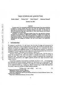
Fig. 1. A graph of a sentence length sampler autocorrelation function. Fig. 1 emonstrate a graph of a sampler autocorrelation function which is computed on seniences lengths (measured in words number) of a text "Alice in Wonderland" [2]. The number of sentences
26.5
is n = 1428. In this example values r(k) are not large, for example, r(15) = 0.0336, therefore J a r ( 1 5 ) = 1.263 . It does not a reason to neglect the independencehypothesis. At the same time one can note a significant correlation between the sequential values r(k). To explicate this correlation we introduce a normalized sum qK of products of sequential values r(k):
5K=1y -4 + -
n - 2z 1 r(2i - 1>4=
- r(2i).
i=l
Note that due to Theorem 1 summands of 5K converge as n - K
+ CD to
a distribution of two
independent standard noma1 random variables, and due to the Central Limit Theorem . J2/K gK converges to a standard nornal law, if K = K ( n ) is an enough slowly growing function.
In our example K=357, 5K =496.2, J2/K-gK=37.14. Thus .\IZ/K.gK is in the area of large deviations, and we must use theorem on large deviations for the correct calculation of the significance level. 4. Large deviations
If the function K = K ( n ) grows enough slowly then we can study large deviations of 5; instead of large deviations of 5 K .Here
random variables q,,q2,...have standard normal distribution. 5; is a sum of [ K / 2 ] independent random variables identically distributed with qq2. Check Cramer condition [3] and calculate Laplace transform of the random variable qlq2.
for
I A I