DEPICTING FUZZY SOIL CLASS UNCERTAINTY USING PERCEPTION-BASED COLOR MODELS 1
James E. Burt1 A-Xing Zhu2,1 Mark Harrower1 Department of Geography, University of Wisconsin-Madison, Madison, Wisconsin, USA 53706 Email:
[email protected],
[email protected]
2State Key Laboratory of Resources and Environmental Information Systems, Institute of Geographical Sciences and Natural Resources Research, Chinese Academy of Sciences, No. 11 Datun Road, Anwai, Beijing, China 100101 The hardening process assigns the pixel to class 2, but obviously exaggerates its membership in that class while deflating membership in the other three classes. Exaggeration uncertainty indexes this using the departure from full membership in class 2:
ABSTRACT: Fuzzy classification typically assigns pixels or polygons to a category with some estimated degree of uncertainty. There are strong incentives for depicting uncertainty along with category, and numerous authors have recommended that this be done using progressive desaturation of the entity’s color with increasing uncertainty. This paper shows that such recommendations cannot be naively applied using color models widely used in computer graphics because colors equally “saturated’’ do not appear equally certain. We demonstrate that models based on color perception are preferred, particularly if one wishes to compare uncertainties across classes. We discuss geometrical complications arising with perceptual models that are not present with models closely tied to hardware. An algorithm for selecting colors is presented and illustrated using the OAC-OCS (Ljg) model.
E = 1 – Max(Pi) = 1 - 0.4 = 0.6
(1)
That is, in claiming sole membership in class 2, we exaggerate by 60%. Alternatively, the ignorance uncertainty is I = - 1/log(n) Σ Pi log(Pi) =
0.92
(2)
indicating that this pixel has relatively uniform membership in multiple categories. That is, I informs a user that the pixel might reasonably be assigned to other classes.
Keywords: uncertainty, classification, visualization Regardless of how uncertainty is measured, methods are needed for mapping categories along with the associated uncertainties. This paper considers methods for accomplishing that in ways that are optimal from a perceptual standpoint. We should emphasize that although the discussion is motivated by fuzzy classification, the following applies to chloropleth mapping in general, whenever a normed uncertainty value can be assigned to attribute data. That is, the only requirement is that uncertainty be expressed on the same finite scale for all classes. (Note that this excludes standard errors and similar measures which do not have a natural upper bound.)
1. INTRODUCTION 1.1 Background Fuzzy classification is becoming routine in remote sensing and related aspects of geographic information science. Unlike traditional classification, which implicitly assumes entities are members of a single class, fuzzy classifiers admit membership in multiple categories. The classification process occurs when pixels or polygons are assigned through hardening to a single category, namely the category of highest membership. Our application is in the area of soil prediction, where we first estimate the membership of pixels in a set of nominal soil categories [10]. In this case hardening assigns a single soil category to each pixel.
1.2 Problem Our goal is effective presentation of category and uncertainty on the same map. This is hardly a new problem, and various authors have suggested that decreasing color saturation can be used to indicate progressively larger amounts of uncertainty [see 2, 4, 5]. That is, an entity having no uncertainty appears as a fully saturated color, whereas total uncertainty is rendered in a monochrome color. This can be readily accomplished using tools available in common mapping, GIS, and illustration software, almost all of which provide the ability to define color in HSV, HLS, or a similar system that explicitly contains “saturation” as a variable [1]. However, such color systems have been developed for
Typically, along with the category value, an uncertainty value is attached to each entity. As discussed in [9], the uncertainty value might be a measure of the distance between the classified entity and a prototype defined for the most-similar category (exaggeration uncertainty), or it might index the degree to which the entity has membership in multiple categories (ignorance uncertainty). Consider, for example, a vector indicating a pixel’s similarity (P) to 4 classes: Hardening P = (0.2, 0.4, 0.1, 0.3) --------------> (0, 1, 0, 0) 1
provides a better basis for rendering uncertainty than methods based on hardware-related models such as HSV or HLS.
ease of use, and are not tied to any absolute standard of color or psychophysical response. For example, fully saturated red is mapped to whatever is the most “pure” red the current display device can produce, without reference to any color standard nor is there any consideration of how that color will be perceived. Thus there is no guarantee that a 50%-saturated red will appear equally uncertain as a 50%-saturated yellow. In fact, because the HSV and HLS systems conflate luminance (lightness) and saturation, we can be sure that they will not. This is seen in Figure 1, which shows the top of the HSV cone. If the model were perceptually accurate, luminance would decrease outward in concentric rings. The appearance of brighter and darker “rays” of luminance in some directions indicates that this model fails on perceptual grounds.
Application of this approach is complicated by the fact that the universe of possible colors in these models is bounded by an irregular 3-dimensional solid. For example, Figure 2 shows slices of the L*a*b* system for a few values of L*.
Figure 2. Cross-sections of the L*a*b* space for various luminance values.
Figure 1. Full-value HSV colors.
It, like Figure 3, was produced by a program available as ftp:\\solim.geography.wisc.edu\OUT\ColorSlices.exe. The cross-sections are centered with respect to one-another, meaning that the gray points (a* = b* = 0) are in the center of each square. Figure 3 shows similar cross-sections for the Munsell system. Note that in both of these systems, one can move radially from the origin with little or no apparent change in luminance. Thus, in contrast to what is seen in Figure 1, these systems are much closer to offering saturation values proportional to perceived uncertainty.
The basic difficulty is that in some directions (i.e., for some hues) a unit change in saturation gives a larger change in luminance than others. The result is that apparent certainty—or equivalently, the perceptual distance from white —varies nonuniformly with hue. 2. METHOD Fortunately, a number of perception-based color models exist, including Munsell, the CIE systems L*a*b* and L*u*v*, and Ljg system of the Optical Society of America [3, 7]. These systems are similar in that they are tied to a prescribed color standard, and thus the colors associated with a particular point in the color model are not dependent on the properties of the display device. These are also similar in that all are 3-dimensional models in which a unit change in any direction is supposed to give a uniform perceptual change. Finally, all contain a luminance axis perpendicular to two other orthogonal axes that in combination yield the hue of a color. Monochrome colors are found along the luminance axis, and increasing saturation is found along radial lines in any plane of constant luminance. Thus two points equidistance from the luminance axis will in principle have equal perceived uncertainty. In the method proposed here, colors assigned to each soil category will be located on a ray originating at the luminance axis. Total uncertainty will be indicated by points at the origin, with colors for progressively more certain pixels chosen progressively farther along the ray. We propose that this approach
Figure 3. As for Figure 2, but for the Munsell system. Note that in Figures 2 and 3 the maximum distance possible, i.e., the maximum saturation possible, depends 2
heavily on luminance and hue. Similar conclusions hold for the L*u*v* and Ljg systems (not shown). We propose that for any luminance value, pixels with complete certainty (unity) should be located as far as possible from the monochrome point. This will obviously maximize the range in perceived uncertainty, and thereby maximize the visual resolution in uncertainty. Another requirement is that any two pixels having the same uncertainty should be as far as possible from each other in the color space. Taken together, these requirements mean that fully saturated colors will be equally spaced along a circle centered on the origin. Reflecting this, our basic algorithm is as follows:
3. IMPLEMENTATION and RESULTS 3.1 Basic Method The algorithm has been implemented as a C++ program for MS-Windows and is available from ftp:\\solim.geography.wisc.edu\OUT\ColorBars.exe. The program computes colors for a variable number of classes in the L*u*v*, L*a*b* and Ljg models, as well as for HSV. [We have not implemented Munsell because as a discrete model, it contains gaps that could only be filled by interpolation. Such interpolated colors would not be part of the color model, and we are reluctant to invent them.]
Given the number of classes n (n > 1): 1) Define the angle between hues θ = 360o/n 2) Select a luminance value L* or L. 3) Search for optimum equally spaced directions α1, α2, … αn where αi = αi-1 + θ: a. Initialize Smax = 0 b. For τ = 1o, 2o, … θ try α1= τ, α2= τ+θ, ... c. Find Smin, the minimum saturation possible for α1, α2, … αn. If Smin > Smax, save τ as τopt and assign Smin = Smax. d. Let αi = i (τopt), i = 1, 2, … n.
The search algorithm was implemented as indicated, with no attempt at optimization. Therefore the slow search method, along with the complexities of converting from perceptual coordinates to RGB, means the approach cannot be used as coded in real-time applications. In particular, on a personal computer the program requires 2-3 seconds to identify and display a full suite of colors for all four models. However, in most instances the classification process generating the map data will be very slow by comparison, thus efficiency in choosing colors is not a factor.
This process gives n colors on the circumference of a circle whose radius is just small enough to ensure that all n colors are realizable. As an example, consider Figure 4, which shows the colors that result for a map with n = 3 (three soil classes).
Figure 5 is an example of the output showing just the panels for the Ljg and HSV models. Moving horizontally across the color bars at constant saturation, there would ideally be no change in perceived uncertainty. At least for the authors, the Ljg bars come significantly closer to that ideal than the HSV bars shown in Figure 5.
Figure 4. Cross-section of Ljg for L = 50 showing optimum color choices for 3 soil classes. Pixels for a class would be chosen from colors along rays connecting a point and the origin (black dot). The dots indicate colors that would be used for pixels with no uncertainty. All are equidistant from gray, and thus have equal saturation. However, only one of them—the upper, left point—has the maximum saturation possible for its hue. The other two points are somewhat under-saturated relative to what is possible. The fact that the circle crosses outside the envelope of possible colors is of no consequence because a map would contain only colors along rays from the dots to the origin.
Figure 5. Color gamuts from the Ljg and HSV models for a four-category map. We have done no formal testing, but our examination of results for n = 2, 3, …12 confirms that three 3
on and off, as with 3dMapper.
perceptual models always out-perform HSV in this regard.
3.2 Enhancements Our primary result, therefore, is to provide evidence that the theoretical advantages of perception-based models very likely translate into actual advantages. We recognize that the question will only be answered definitively by a carefully controlled study using human subjects. We believe that our results provide support for such future studies. In addition, our subjective analysis is is that suggests that Ljg model is preferred, but we are not prepared to claim its superiority over the two CIE models. Again, that needs to be answered by more study. In addition, such studies need to investigate whether continuous variation in saturation is best. It might be that only a few saturation classes would be preferable.
There are two obvious enhancements, both of which are useful for increasing the dynamic range of colors available. As we have indicated, each class has a range of colors lying along a line running from achromatic to the maximum possible saturation, which is the same for all classes. To increase the range of colors, we need to lengthen that line. One obvious way to increase the range is to search for a luminance value that give as large a radius as possible. In other words, for a given n, we need to find an L* or L that maximizes the radius Smax. That is easily accomplished by replacing Step (2) in the algorithm with a line search along the luminance axis. For every trial point along the axis, we examine the cross-section to find the largest radius possible for that luminance. The maximum over all luminance values reveals the optimum luminance.
As another example, consider Figure 6, which results from applying the method to a ten-class soils map displayed using 3dMapper [11]. Note that the combination of class and uncertainty provides important information that would be hard to obtain from either map
Another way to increase the range is to use white as the origin of every color bar. That is, instead of holding luminance fixed along the color bar, we allow luminance increase, with white rather than some gray level as the color associated with maximum uncertainty. Geometrically, we allow the bars to slant upward from the optimum luminance to white, which obviously lengthens each bar (see Figure 7.)
Figure 6. A combined category/uncertainty map. alone. For example, in many locations there is a gradual transition through zones of uncertainty, indicating intermediate soils that do not fall neatly into any category. But in other places there is a sharp break from relatively certain to uncertain following abrupt changes in bedrock control. Notice also that this map raises the question of whether or not synthetic hill-shading is advantageous. It obviously provides important clues about landform, but shadows move pixel colors down the luminance axis, which has the potential to be interpreted as increasing uncertainty. Our strong inclination is therefore to provide shading only in interactive environments, where the effective sun position can be easily varied, and even in those instances we recommend providing shading as an option that can easily be toggled
Figure 7. Color bars forced to terminate on white. Note that because they cross luminance values, it is possible for a bar to exit the volume of realizable colors. Our code checks for that, and displays a warning message when it occurs. As a practical matter, this might not be a significant issue---at least we did not encounter the problem in any of our testing. This follows from the fact that the intersections of the color volumes and a plane running through the luminance axis are not too far from convex. (Figure 2 gives some hint of that.) Note also that the color bars could be extended by terminating 4
them at a lower luminance value, that is, at a darker gray or even black. Our subjective evaluation is that this tends to overly obscure differences in hue to the point that the base class is becomes difficult to ascertain.
6. REFERENCES [1] Foley, J.D., A.van Dam, S.K. Feiner and J.F. Hughes, Computer Graphics: Principles and Practice (Second Edition in C), Addison-Wesley, 1996.
4. CONCLUSIONS [2] Goodchild, M., B. Buttenfield, and J. Wood, "Introduction to visualizing data uncertainty". Chapter 15 in Visualization in Geographical Information Systems, H.M. Hearnshaw and D. J. Unwin (eds.). Chichester: Association for Geographic Education (Wiley), 1994.
We argue that perceptual color models such as L*u*v* and Ljg are better choices for displaying class uncertainty than other more commonly used models such as HSV or HLS. Although they are not suitable for real-time display, perceptual models have a strong advantage in maps whose categories and uncertainties are fixed. That is, they are indisputably superior on theoretical grounds because they are designed to give the appropriate psychophysical response. The informal evaluations reported here are entirely consistent with that advantage, but further work using human subject testing is needed for confirmation. Human testing is also needed to examine an assumption that we have not discussed, namely whether or not saturation in a perceptual model scales linearly to perceived uncertainty. For example, we wonder if 40% saturation is perceived to be twice as uncertain as 20% saturation. The models are designed so that the perceived colors have the proper relationship, but we do not know how color is mapped to the perception of uncertainty.
[3] Hunt, R.W.G., The Reproduction of Color (5th ed.). Kingston-upon-Thames, England: Fountain, 1995. [4] Leitner, M. and B. Buttenfield, “Guidelines for the display of attribute uncertainty”, Cartography and Geographic Information Science, 27: 3-14, 2001. [5] McEachren, A.M., “Visualizing uncertain information”, Cartographic Perspectives, 13: 10-19, 1992. [6] Nemani, R.R., C.D. Keeling, H. Hashimoto, W.M. Jolly, S.C. Piper, C.J. Tucker, R. B. Myneni, S.W. Running, “Climate-driven increases in global terrestrial net primary production from 1982 to 1999”, Science, 300: 1560-1563, 2003.
It is important to emphasize that our study is narrowly focused on pixel-level display of uncertainty. Accordingly, it considers only saturation as a visual variable to be manipulated in conveying uncertainty. Other variables (e.g. texture, crispness, resolution) cited as useful for uncertainty cannot be applied at the pixel level [see 8, p. 242-249]. We do not mean to imply that saturation is the best variable for rendering uncertainty in other situations, such as when mapping point or boundary placement. Rather, our goal has been to provide guidance regarding how saturation can best be used for pixel uncertainty, given that it appears to be the only logical candidate.
[7] Nickerson, D., “OSA uniform color scale samples: a unique set”, Color Research and Application, 6: 7-33, 1981. [8] Slocum, T.A., Thematic cartography and visualization. New York: Prentice-Hall, 1999. [9] Zhu, A.X., “Measuring uncertainty in class assignment for natural resource maps using a similarity model”, Photogrammetric Engineering & Remote Sensing, 63: 1195-1202, 1997. [10] Zhu, A.X, B. Hudson, J.E. Burt , K. Lubich, and D. Simonson D., “Soil mapping using GIS, expert knowledge, and fuzzy logic”, Soil Science Society of America Journal, 65: 1463-1472, 2001.
We close by noting that in addition to situations like those described here, where uncertainty is generated as part of some discrete classification process, our method has utility when a continuous attribute value is imprecise. For example, in [6] purity of color was used to indicate the relative contribution of three variables to net ecosystem productivity. We believe that a continuum anchored in a perceptual model is appropriate for such maps.
[11] 3dMapper: Software for 3-d landscape visualization and mapping, Terrain Analytics, L.L.C.. Available from www.TerrainAnalytics.com.
5. ACKNOWLEDGEMENTS The financial and logistical supports from the USDA Natural Resources Conservation Service and the Chinese Academy of Sciences through its “One-Hundred Talent Program” are gratefully acknowledged.
5