Depth of Field Postprocessing For Layered Scenes Using Constant-Time Rectangle Spreading
Todd Jerome Kosloff Michael Tao Brian A. Barsky
Electrical Engineering and Computer Sciences University of California at Berkeley Technical Report No. UCB/EECS-2008-187 http://www.eecs.berkeley.edu/Pubs/TechRpts/2008/EECS-2008-187.html
December 30, 2008
Copyright 2008, by the author(s). All rights reserved. Permission to make digital or hard copies of all or part of this work for personal or classroom use is granted without fee provided that copies are not made or distributed for profit or commercial advantage and that copies bear this notice and the full citation on the first page. To copy otherwise, to republish, to post on servers or to redistribute to lists, requires prior specific permission.
Depth of Field Postprocessing For Layered Scenes Using Constant-Time Rectangle Spreading Todd J. Kosloff∗
Michael Tao†
Brian A. Barsky‡
University of California, Berkeley Computer Science Division Berkeley, CA 94720-1776
University of California, Berkeley Computer Science Division Berkeley, CA 94720-1776
University of California, Berkeley Computer Science Division and School of Optometry Berkeley, CA 94720-1776
Figure 1: Spreading vs. Gathering. Left: Gathering leads to sharp silhouettes on blurred objects. Right: Spreading correctly blurs silhouettes. This scene uses two layers, one for the background, one for the foreground.
A BSTRACT Control over what is in focus and what is not in focus in an image is an important artistic tool. The range of depth in a 3D scene that is imaged in sufficient focus through an optics system, such as a camera lens, is called depth of field. Without depth of field, everything appears completely in sharp focus, leading to an unnatural, overly crisp appearance. Current techniques for rendering depth of field in computer graphics are either slow or suffer from artifacts and limitations in the type of blur. In this paper, we present a new image filter based on rectangle spreading which is constant time per pixel. When used in a layered depth of field framework, it eliminates the intensity leakage and depth discontinuity artifacts that occur in previous methods. We also present several extensions to our rectangle spreading method to allow flexibility in the appearance of the blur through control over the point spread function. Index Terms: I.3.3 [Computer Graphics]: Picture/Image Generation-display algorithms, bitmap and frame buffer operations, viewing algorithms— 1
I NTRODUCTION
1.1
Background
Control over what is in focus and what is not in focus in an image is an important artistic tool. The range of depth in a 3D scene that is imaged in sufficient focus through an optics system, such as a camera lens, is called depth of field. This forms a swath through a 3D scene that is bounded by two planes that typically are both parallel to the film/image plane of the camera. Professional photographers or cinematographers often control the focus distance, aperture size, and focal length to achieve desired effects in the image. For example, by restricting only part of ∗ e-mail:
[email protected]
† e-mail:
[email protected]
a scene to be in focus, the viewer or the audience automatically attends primarily to that portion of the scene. Analogously, pulling focus in a movie directs the viewer to look at different places in the scene, following the point of focus as it moves continuously within the scene. Rendering algorithms in computer graphics that lack depth of field are in fact modeling a pinhole camera model. Without depth of field, everything appears in completely sharp focus, leading to an unnatural, overly crisp appearance. Techniques for rendering depth of field in computer graphics are well known, but they all are either slow, or suffer from artifacts or limitations. Distributed ray tracing [9] can render scenes by directly simulating geometric optics, resulting in high quality depth of field effects. However, many rays per pixel are required, leading to slow render times. Post-processing, which adds blur to an image that was rendered with everything in perfect focus, is the alternative for efficiently simulating depth of field. 1.2
Goals
A good depth of field postprocess method should meet the following criteria: 1. Allows the amount of blur to vary arbitrarily from pixel to pixel, as each pixel can lie at a different distance from the focus plane. 2. Achieves high performance, even for large amounts of blur. 3. Allows control over the nature of the blur, by allowing flexibility in choice of the PSF (Point Spread Function). 4. Avoids depth discontinuity artifacts. Some fast methods lead to jarring discontinuities on the silhouettes of blurred objects.
‡ e-mail:
[email protected]
5. Avoids intensity leakage artifacts. Some fast methods lead to a blurred background leaking on top of an in-focus foreground. Intensity leakage is not physically correct and takes away from the realism of the image.
objects will incorrectly exhibit sharp silhouettes. Scofield shows how to solve this problem in the case of axis-aligned planar objects using layering [33]. Each object is placed into a layer, along with an alpha matte. The layers and alpha mattes are blurred using convolution via FFT, and the blurred objects are composited using alpha blending with the blurred alpha mattes. In this paper we describe a novel set of image filters suitable for efficiently extending Scofield’s method to nonplanar layers. As a prerequisite to using a layered method, the scene in question must be decomposed into layers. We assume that the decomposition has already been performed, either manually or automatically, and describe how to perform depth of field postprocessing using these layers. 3
Figure 2: A scene blurred using our basic square spreading method. Left: focus on wall. Right: focus on cone.
In this paper, we describe new image filters that, when used on layered scenes, simultaneously meet all of these criteria. Spatially varying image filters can typically be characterized as utilizing either spreading or gathering, as will be explained in the next section of this paper. Existing fast blur filters generally use gathering, which is physically incorrect, and leads to noticeable flaws in the resulting image. In this paper, we show that spreading removes these flaws, and can be very efficient. We describe a novel fast spreading blur filter, for use in depth of field for layered scenes. Our method takes inspiration from the summed area table (SAT) [10], though our method differs substantially, in that a SAT is fundamentally a gather method while our method uses spreading. We can characterize the appearance of the blur in an image by the PSF, which describes how a point of light in the scene would appear in the blurred image. Our basic method uses rectangles of constant intensity as the PSF. To allow for more flexible choice of PSFs, we describe two alternate extensions to our method: one that uses constant-intensity PSFs of arbitrary shape, and another that hybridizes any fast blur method with a slower, direct method that allows PSFs of arbitrary shape and intensity distribution. In this way, we achieve a controllable tradeoff between quality and speed. 1.3 Summary of Contributions This paper makes the following contributions to the problem of depth of field postprocessing of layered scenes. 1. We show that spreading filters do not lead to the depth discontinuity artifacts that plague gathering methods. Note that the use of layers solves the intensity leakage problem when used with either gathering or spreading methods. 2. We show that Crow’s summed area table, fundamentally a gather method, can be transformed into a spreading method. 3. We extend the SAT-like method to handle constant-intensity PSFs of arbitrary shape, at modest additional cost. 4. We show how to hybridize any fast spreading filter with arbitrary PSFs according to a controllable cost/quality tradeoff. 2
D EPTH OF F IELD P OSTPROCESSING OF L AYERED S CENES When blurring an image of a scene using a linear filter, blurred background objects will incorrectly leak onto sharp foreground objects, and sharp foreground objects overlapping blurred background
S PREADING
VS .
G ATHERING
The process of convolving an image with a filter can equivalently be described as spreading or gathering. Spreading means each pixel in the image is expanded into a copy of the filter kernel, and all these copies are summed together. Gathering means that each pixel in the filtered image is a weighted average of pixels from the input image, where the weights are determined by centering the filter kernel at the appropriate pixel. When we allow the filter kernel to vary from pixel to pixel, spreading and gathering are no longer equivalent. In any physically plausible postprocess depth of field method, each pixel must spread out according to that pixel’s PSF. Each pixel can have a PSF of different size and shape, so we designed our filter to vary from pixel to pixel. Fast image filters typically only support gathering, so fast depth of field postprocess methods generally use gathering, despite the fact that spreading would produce more accurate results. We present a depth of field postprocess approach for layered scenes. For example, consider a scene with a foreground layer and a background layer. Both layers are blurred, and are then composited with alpha-blending. Blurring and compositing layers for depth of field postprocessing was first developed by Scofield [33]. However, Scofield blurred via convolution, which limited each layer to only a single amount of blur; this is accurate only for planar, screenaligned objects. Despite this limitation, Scofield’s method is free of depth discontinuity and intensity leakage artifacts. We wish to use spatially-variant blur instead of convolution, to extend Scofield’s method to scenes where the layers are not necessarily planar or axis-aligned. We initially considered using Crow’s summed area table (SAT) as the image filter, since SATs run in constant time per pixel and allow each pixel to have an independently chosen filter size. In any given layer, some of the pixels will be opaque, and others will be completely transparent. For the sake of discussion, we ignore semitransparent pixels, though these are allowed as well. To generate the blurred color for an opaque pixel, we look up the depth value of the pixel, and determine a filter size using a lens model. We then perform a SAT lookup to determine the average color of the filter region. Unfortunately, it is not straightforward to determine a blurred color for a transparent pixel, as transparent pixels correspond to regions outside of any object, and thus do not have depth values. Depth values must be extrapolated from the opaque pixels to the transparent pixels, a process that generally only approximates the correct result, and requires additional computation. Barring such extrapolation, transparent pixels must be left completely transparent. Consequently, pixels outside of any object remain completely transparent, even after blurring, even if said pixels are immediately adjacent to opaque pixels. Visually, this results in a sharp discontinuity in the blurred image, along object silhouettes (Figure 1, left). We refer to these problems as depth discontinuity artifacts. It is important to note that this problem with transparent pixels does not occur with methods that blur by breaking the image into layers which are then approximated with spatially uniform blur [24], [2], as spatially uniform blur does not consider depth values at all, after
discretization. However, blurring by discrete depth simply replaces depth discontinuity artifacts with discretization artifacts [5]. A better option is to use a spreading filter. When an object is blurred by spreading, opaque pixels near silhouettes will spill out into the adjacent region, yielding a soft, blurred silhouette (Figure 1, right). This is a highly accurate approximation to the partial occlusion effect seen in real depth of field. This need for spreading filters motivates the constant-time spreading filter presented in this paper. 4
P REVIOUS W ORK
Potmesil and Chakravarty [29] developed the first ever depth of field rendering algorithm. They used a postprocess approach that employed complex PSFs derived from physical optics. Their direct, spatial domain filter is slow for large blurs. Cook [9] developed distributed ray tracing, which casts many rays per pixel in order to achieve a variety of effects, including depth of field. Kolb [23] later showed how distributed ray tracing can be used to simulate particular systems of camera lenses, including aberrations and distortions. Methods based on distributed ray tracing faithfully simulate geometric optics, but due to the number of rays required, are very slow. The accumulation buffer [18] uses rasterization hardware instead of tracing rays, but also becomes very slow for large blurs, especially in complex scenes. Scheuermann and Tatarchuk [32] developed a fast and simple postprocess method, suitable for interactive applications such as video games. However, it suffers from depth discontinuity artifacts, due to use of gathering. They selectively ignore certain pixels during the gathering, in order to reduce intensity leakage artifacts, though, due to their use of a reduced resolution image that aggregates pixels from many different depths, does not eliminate them completely. Their method does not allow for a choice of point spread function; it produces an effective PSF that is a convolution of a bilinearly resampled image with random noise. Our methods allow a choice of PSF, and eliminate the depth discontinuity artifact. Krauss and Strengert [24] use pyramids to perform fast uniform blurring. By running the pyramid algorithm multiple times at different pyramid levels, they approximate a continuously varying blur. Unlike our method, their method does not provide a choice of PSFs, but rather produces a PSF that is roughly Gaussian. Bertalmio et al. [7] showed that depth of field can be simulated as heat diffusion. Later, Kass et al. [22] use a GPU to solve the diffusion equation for depth of field in real time using an implicit method. Diffusion is notable for being a blurring process that is neither spreading nor gathering. Diffusion, much like pyramids, inherently leads to Gaussian PSFs. Mulder and van Lier [26] used a fast pyramid method at the periphery, and a slower method with better PSF at the center of the image. This is somewhat similar to our hybrid method, but we use an image-dependent heuristic to adaptively decide where the high quality PSF is required. Many other methods exist that achieve fast depth of field, such as [13], [25], [30] and [35], though they all suffer from various artifacts and limitations. The use of layers and alpha blending [28] for depth of field was introduced by [33]. We also use this layering approach, though our image filters offer significant advantages over those used by Scofield. Barsky showed in [6] and [5] how to use object identification to allow objects to span layers without artifacts at the seams. Other methods exist as alternates to layers, such as Catmull’s method for independent pixel processing [8], which is efficient for scenes composed of a few large, untextured polygons, and Shinya’s ray distribution buffer [34], which resolves intensity leakage in a very direct way, at great additional cost. We choose to use layers due to their simplicity and efficiency.
For a comprehensive survey of depth of field methods, please consult Barsky’s [3] [4] and Demers’ [11] surveys. The method presented in this paper uses ideas similar to Crow’s summed area table [10] originally intended for texture map antialiasing. Other constant-time image filters intended for texture map anti-aliasing methods include [14] and [16]. We build our method along the lines of Crow’s, as it is the simplest. The well known Huang’s method [21], (cost linear to kernel size), and extended, (cost constant to kernel size), [27] are very fast algorithms to compute the square blur. As the window of the kernel moves to the next pixel, the new pixel values of the window are added to the summation while the old values are subtracted from the summation. By storing the summation of the columns into memory, the process of calculating the blurred value becomes a constant computation. Unfortunately, the limitations of these methods is that the kernel must be rectangular and at a constant size. With these limitations, the Huang’s and the extended method are not favorable for depth of field blurring. Finally, the Fast Fourier Transform (FFT) is a traditional fast method for blurring pictures via convolution, but only applies where the amount of blur throughout an image is constant. Therefore many FFTs are required if we want the appearance of continuous blur gradations. When many FFTs are required, we no longer have a fast algorithm, even if the FFTs are performed by a highly optimized implementation such as FFTW [15]. Therefore, we do not use FFTs in our method. 5 5.1
C ONSTANT T IME R ECTANGLE S PREADING Motivation For Examining the Summed Area Table
We draw inspiration from Crow’s summed area table (SAT). We base our method on the SAT rather than on one of the other table methods, because of the following speed and quality reasons. Table-based gather methods can be used in a setting where the table is created offline. This means that it is acceptable for table creation to be slow. Consequently, some of these methods do indeed have a lengthy table creation phase. [14], [16]. However, the summed area table requires very little computation to create, and so can be used online [20]. With a SAT, we can compute the average color of any rectangular region. Both the size and location of the region can be specified with pixel-level precision. Other methods, such as [16] and [14], give less precise control. While summed area tables have beneficial qualities, they can only be used for gathering, requiring us to devise a new method that can be used for spreading. Furthermore, SATs have precision requirements that grow with increased image size. Our rectangle spreading method does not inherit these precision problems, as the signal being integrated includes alternating positive and negative values. 5.2
Our Basic Rectangle-Spreading Method
First, we must create an array of the same dimensions as the image, using a floating point data type. We will refer to this as table. After initializing the array to zero, we enter Phase I of our method [Figure 4]. Phase I involves iterating over each pixel in the input image, consulting a depth map and camera model to determine how large the circle of confusion is, and accumulating signed intensity markers in the array, at the corners of each rectangle that we wish to spread. Thus we tabulate a collection of rectangles that are to be summed together to create the blurred image. At this point, the array contains enough information to construct the blurred image, but the array itself is not the blurred image, as only the corners of each rectangle have been touched. To create the blurred image from the array, we need Phase II of our method [Figure 5]. Phase II is similar to creating a summed
Figure 3: For every image input, there are two input buffers (A)- the image channel as an input and the normalization channel, which is the size of the image and contains pixels of intensity 1.0. In Phase I (B), for each pixel, we read the value of the pixel and spread the positive and negative markers accordingly on to the table (c). In Phase II (D), there is an accumulator (shown in orange) that scans through the entries of the tables from left to right, top to bottom. The accumulated buffer (E) stores the current state of the accumulator. Phase II is equivalent to building a summed area table of the table (c). In phase III (F), for each entry at i and j, we divide the image’s accumulated buffer by the normalization channel’s accumulated buffer to obtain the output of the image (G).
+
+
-
-
-
+
Figure B Spreads pixels into rectangles by marking the corners.
Figure A We will be blurring this simplified image.
-
+ +
-
+
-
+
+
+
-
-
+
+
-
+
-
-
+
+
-
-
+
First Pixel
Second Pixel
-
+ -
area table from an image. However, the input to Phase II is a table of accumulated signed intensities located at rectangle corners, whereas the input to a summed area table creation routine is an image. Furthermore, the output of Phase II is a blurred image, whereas the output of a summed area table creation routine is a table meant to be queried later. A summary of the entire blur process is illustrated in Figure 3.
+ +
Third Pixel
Figure 4: Phase I: Accumulating
//This code is for a single color channel, //for simplicity. //In a real implementation, R,G,B and A channels //must all be blurred by this same process. //Fast rectangle spreading: Phase I. float table[width][height]; float area; //zero out table (code omitted) //S is the input image (S stands for sharp) for(int i=0; i