June 1, 2005 / Vol. 30, No. 11 / OPTICS LETTERS
1303
Depth-of-focus reduction for digital in-line holography of particle fields Weidong Yang, Alexander B. Kostinski, and Raymond A. Shaw Department of Physics, Michigan Technological University, 1400 Townsend Drive, Houghton, Michigan 49931 Received January 3, 2005 Poor axial precision caused, in part, by large depth of focus 共兲 has been a vexing problem in extraction of particle position from digital in-line holograms. A simple method is proposed to combat this depth-of-focus difficulty. The method is based on decoupling of size and position information. With d , ⌬, and being particle diameter, CCD pixel size, and the wavelength, respectively, our main theoretical result is the reduction of from ⬃ d2 / to ⬃ ⌬2 / for particles of known size. This result is confirmed in laboratory experiments with holograms of calibrated glass spheres. © 2005 Optical Society of America OCIS codes: 090.0090, 120.3940.
The transition from film-based to digital holography, fueled by the ever-increasing speed of digital recording and computation, has opened up exciting applications such as three-dimensional particle image velocimetry.1,2 Here we examine the in-line version of digital holography because of its simplicity and practical appeal.3–5 Specifically, we consider the problem of extracting particle positions from in-line digital holograms, which is particularly important for such applications as particle image velocimetry1,2 and measurements of particle spatial statistics.6 Many methods of particle field extraction have been proposed in the literature,5,7–15 but most exhibit poorer axial than transverse precision. Particle positions along the optical axis typically are determined by searching for extrema in the reconstructed intensity, amplitude, or complex variance.12–15 Therefore in digital holography such algorithms are subject to the depth-of-focus constraint:2,5,16
⬃ d2/,
共1兲
where d and are the particle diameter and the illuminating wavelength, respectively. For example, a particle diameter of 23 m and ⬃ 0.5 m result in of ⬃1.1 mm, or 46d. Clearly, the quadratic dependence on the particle size makes the resolution of large particles problematic. We now proceed to demonstrate that the depth-of-focus difficulty can be overcome for particles of known size. As a preliminary, observe that expression (1) implies that as d / decreases relative axial precision 共 / d兲 improves. Hence the point particle case is ideal. This suggests that disentangling the effects of particle size from those of its location might deliver the desired result. Crudely, the position information is encoded in the relative spacings between the hologram fringes, and the size affects the relative brightness of the rings. Therefore restoring the ring brightness to the point source pattern may result in a much shorter depth of focus. This is indeed the case, and we now describe the mathematical implementation of this idea. We then conclude with an experimental confirmation of the results. 0146-9592/05/111303-3/$15.00
The typical digital in-line holographic configuration contains only collimating optics and a CCD that will record the interference intensity pattern between the collimated on-axis reference light and the forward-scattering light from the particles. If the intensity pattern at the CCD hologram plane 共s , t兲 is denoted i共s , t兲, then, under Fresnel approximation, the reconstructed scattered light field on any interrogation plane 共u , v兲 at distance −z (relative to the hologram plane) can be written as ez共u,v兲 =
冕冕 ⬁
⬁
−⬁
−⬁
关1 − i共s,t兲兴h−z共u − s,v − t兲dsdt, 共2兲
where hz共u − s , v − t兲 = 共1 / jz兲exp兵共j / z兲关共u − s兲2 + 共v 2 − t兲 兴其 and the reference plane wave is normalized to 1. The convolution can be performed equivalently through ez共u,v兲 = F−1兵关␦共, 兲 − I共, 兲兴H−z共, 兲其,
共3兲
where F−1兵 其 denotes the inverse Fourier transform and I and Hz are the Fourier-transform counterparts of i and hz in the Fourier domain 共 , 兲, respectively. Specifically, ␦ is the Dirac delta function and Hz共 , 兲 = exp关−jz共2 + 2兲兴.17 We now seek a Fourier-domain filter that will allow us to remove the effect of the finite particle aperture on the reconstruction estimate of particle location. Assuming that we know the particle size, this is accomplished by defining a filter F共 , 兲 = 1 / P共 , 兲 in which P共 , 兲 is the Fourier transform of the particle aperture function p共x , y兲 in the particle object plane 共x , y兲. Then the new reconstructed field ez⬘共u , v兲 after applying the filter would be ez⬘共u,v兲 = F−1
再
␦共, 兲 − I共, 兲 P共, 兲
冎
H−z共, 兲 .
共4兲
One can appreciate the effect of this filter by considering the scattering from one on-axis spherical particle at distance z0, which can be approximated as Fresnel scattering from an opaque disk.2 The light in© 2005 Optical Society of America
1304
OPTICS LETTERS / Vol. 30, No. 11 / June 1, 2005
tensity in the hologram is i共s , t兲 = 1 − o共s , t兲 − o*共s , t兲 ⬁ ⬁ + 兩o共s , t兲兩2, in which o共s , t兲 = 兰−⬁ 兰−⬁p共x , y兲hz0共s − x , t − y兲dxdy and * denotes the conjugate. After omitting contributions from higher-order terms, the Fourier transform of i共s , t兲 can be approximated as I共 , 兲 = ␦共 , 兲 − P共 , 兲Hz0共 , 兲 − P*共 , 兲Hz* 共 , 兲. From Eq. 0 (4), and omitting the effect of the conjugate of twin images, the new reconstructed field would be ez⬘共u,v兲 ⬇ F−1兵Hz0−z共, 兲其 1 =
j共z0 − z兲
exp兵j共u2 + v2兲/关共z0 − z兲兴其. 共5兲
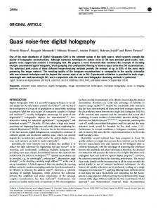
Expression (5) indicates that the reconstructed field after the filter is applied is identical to one generated by a point source, which has an infinitely small depth of focus and a single, infinite intensity peak at z = z0. In practice, however, a limiting factor in digital holography is the finite size of the CCD pixels. The averaging effect of the CCD pixels in recording and in computation smears the fringes that have a spatial period smaller than two pixels and is equivalent to a low-pass filter in the Fourier domain.18 This limiting factor leads to a depth of focus of ⬇ 共2⌬兲2 / , where ⌬ is the CCD pixel size.2 Figure 1 illustrates the improvement in depth of focus gained with this approach. The reconstructions are performed separately based on two simulated inline holograms, one from a d = 30 m particle at 4-cm distance and one from a d = 40 m particle at the same position. The wavelength of illuminating light is 632.8 nm, the hologram (i.e., the detector) is a 512⫻ 512 array with a pixel size of 4.65 m. The dashed–dotted and dashed curves are the reconstructed on-axis intensity profiles (normalized to peak) of the 30- and 40-m particles, respectively, without filtering. If the depth of focus is estimated as
Fig. 1. Simulations of the depth-of-focus improvement. The dashed and dashed–dotted curves are the on-axis normalized intensity profiles for the reconstructed fields of a 40- and a 30-m particle before filtering, respectively; the solid curve with a 170-m depth of focus is the common profile obtained after the filters are applied.
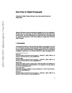
Fig. 2. Experimental demonstration of the depth-of-focus improvement. The top and bottom images in (a) show the normalized intensity distribution on the x – z longitude cross-section plane of reconstructed field of a 30-m particle, before and after filtering, respectively. The dashed– dotted and solid curves in (b) show the on-axis normalized intensity profile before and after filtering in the reconstruction, respectively. The improvement of the depth of focus illustrated in Fig. 1 has basically been achieved.
the profile width at 50% of the peak, the 30- and 40-m particles will show depths of focus of approximately 1.6 and 2.6 mm, respectively. The solid curve is the on-axis intensity profiles for both of the particles reconstructed after applying the filter for each of them. The result is a single-peak intensity profile with a depth of focus of ⬇170 m, an improvement of a factor of ten or greater. It can be seen that the filter pushes the depth of focus to the limit determined only by the pixel size, which in this example is ⬃ 140 m. To demonstrate the effectiveness of this approach in practice, we also compare the reconstruction results using in-line holograms obtained in the laboratory. The experimental system consists of a He–Ne laser, a spatial filter, a collimating lens for illuminating the particles, and a CCD camera for recording the hologram. The CCD contained 1024⫻ 768, 4.65-m square pixels, with 10-bit output. Glass spheres with a diameter of 30 m, with National Institute of Standards and Technology traceable size calibration, were placed on a glass slide ⬃3 cm from the CCD. Figure 2 shows the improvement of the depth of focus by comparing the different intensity reconstruction results with and without applying the inverse filter, based on the same hologram data. Figure 2(a) shows a view of the improvement through the normalized intensity distribution on the x – z longitude
June 1, 2005 / Vol. 30, No. 11 / OPTICS LETTERS
cross-section plane; Fig. 2(b), the on-axis profile. It can be seen not only that the depth of focus improves from 1.75 mm to ⬇270 m but also that the transverse position can be easily identified. Qualitatively, the filter balances (or amplifies) the visibility of the hologram fringes of higher frequencies to the same level of lower frequencies, effectively increasing the numerical apertures.16 It should be noted that, because of division by very small values or zeros in P共 , 兲, this filter is sensitive to additive noise. To avoid this problem we simply modified the filter as
F共, 兲 =
再
1/P共, 兲 P共, 兲 ⬎ threshold 0
otherwise
冎
.
共6兲
In addition, a pixel-size-dependent Fourier-domain Gaussian filter (as described elsewhere15) could be used to smooth the field profiles by removing part of the higher-frequency noise amplified by the filter. It is very likely that there are many other image processing techniques to optimize this filter in terms of its sensitivity to noise, but they exceed the scope of this Letter. In summary, we have proposed and demonstrated through both simulated and laboratory holograms that the large depth of focus believed to be inherent in in-line holograms can be greatly improved by a digital filter to the limit determined only by the pixel size of the detector. This digital filter method relaxes the demands on optical configurations used in in-line holography.16,19,20 However, this method requires that the particle be spherical and requires knowledge of the particle size at the accuracy tolerance of ⬇ ± 5%. Nevertheless, it is effective in applications using seeding particles in which the particle size can
1305
be uniform with high accuracy, such as particle tracking–image velocimetry. This work was supported by National Science Foundation grants ATM99-84294 and ATM01-06271. W. Yang’s e-mail address is
[email protected]. References 1. K. D. Hinsch, Meas. Sci. Technol. 13, R61 (2002). 2. H. Meng, G. Pan, Y. Pu, and S. H. Woodward, Meas. Sci. Technol. 15, 673 (2004). 3. D. Gabor, in Nobel Lectures, Physics 1971–1980, S. Lundqvist, ed. (World Scientific, Singapore, 1992). 4. B. J. Thomson, Proc. SPIE 1136, 308 (1989). 5. C. S. Vikram, Particle Field Holography (Cambridge U. Press, Cambridge, UK, 1992). 6. J. P. Fugal, R. A. Shaw, E. W. Saw, and A. V. Sergeyev, Appl. Opt. 43, 5987 (2004). 7. C. S. Vikram and M. L. Billet, Appl. Phys. B 33, 149 (1984). 8. L. Onural and M. T. Özgen, J. Opt. Soc. Am. A 9, 252 (1992). 9. L. Onural, Opt. Lett. 18, 846 (1993). 10. C. Buraga-Lefebvre, S. Coëtmellec, D. Lebrun, and C. Özkul, Opt. Lasers Eng. 33, 409 (2000). 11. S. Coëtmellec, D. Lebrun, and C. Özkul, Appl. Opt. 41, 312 (2002) 12. S. Murata and N. Yasuda, Opt. Laser Technol. 32, 567 (2000). 13. R. B. Owen and A. A. Zozulya, Opt. Eng. 39, 2187 (2000). 14. G. Pan and H. Meng, Appl. Opt. 42, 827 (2003). 15. C. Fournier, C. Ducottet, and T. Fournel, Meas. Sci. Technol. 15, 686 (2004). 16. F. Liu and F. Hussain, Opt. Lett. 23, 132 (1998). 17. J. Goodman, Introduction to Fourier Optics, 2nd ed. (McGraw-Hill, Boston, Mass., 1996). 18. T. Kreis, Opt. Eng. 41, 1829 (2002). 19. J. Zhang, B. Tao, and J. Katz, Exp. Fluids 23, 373 (1997). 20. J. Sheng, E. Malkiel, and J. Katz, Appl. Opt. 42, 235 (2003).