Digital holography of particle fields: reconstruction by use of ...

Digital holography of particle fields: reconstruction by use of complex amplitude Gang Pan and Hui Meng

Digital holography appears to be a strong contender as the next-generation technology for holographic diagnostics of particle fields and holographic particle image velocimetry for flow field measurement. With the digital holographic approach, holograms are directly recorded by a digital camera and reconstructed numerically. This not only eliminates wet chemical processing and mechanical scanning, but also enables the use of complex amplitude information inaccessible by optical reconstruction, thereby allowing flexible reconstruction algorithms to achieve optimization of specific information. However, owing to the inherently low pixel resolution of solid-state imaging sensors, digital holography gives poor depth resolution for images, a problem that severely impairs the usefulness of digital holography especially in densely populated particle fields. This paper describes a technique that significantly improves particle axial-location accuracy by exploring the reconstructed complex amplitude information, compared with other numerical reconstruction schemes that merely mimic traditional optical reconstruction. This novel method allows accurate extraction of particle locations from forward-scattering particle holograms even at high particle loadings. © 2003 Optical Society of America OCIS codes: 120.7250, 120.3940, 090.1760, 100.3010.

1. Introduction

In many applications involving particle fields there is a pressing need to develop capabilities to measure instantaneous three-dimensional 共3D兲 distributions of small particles dispersed in a flow. For example, in the prediction of raindrop formation in the atmosphere, in the design of fine-spray combustion nozzles, in the production of fine-scale pigments, and in the control of industrial emissions, it is important to model the dispersion, collision, and coagulation of particles suspended in turbulence. Without the spatial and temporal data of particle position and velocity, one cannot develop accurate predictive models or experimentally validate these models and numerical simulations. The capability to dynamically measure 3D position and velocity of a particle will also enable us to track particle motions in a turbulent flow in 3D space and time. When the particles are treated as flow tracers, these measurements provide

The authors are with the Laser Flow Diagnostics Lab, Department of Mechanical and Aerospace Engineering, State University of New York at Buffalo, Buffalo, New York 14260. Received 11 June 2002; revised manuscript received 31 October 2002. 0003-6935兾03兾050827-07$15.00兾0 © 2003 Optical Society of America

valuable information for a Lagrangian description of turbulence.1 Various optical techniques are developed for instantaneous 3D measurement of particle fields including stereoscopic particle tracking,2 defocusing digital particle image velocimetry 共DDPIV兲,3 forward scattering particle image velocimetry 共FSPIV兲,4 and holographic techniques, such as holographic particle image velocimetry 共HPIV兲.5 The stereoscopic approach is based on lens imaging, and hence it can only measure particles in a thin volume. DDPIV uses multiple apertures to obtain multiple images of particles and then determines the 3D position of each particle from the pattern formed by its images. DDPIV essentially uses another format of stereoscopic imaging, and therefore it is restricted in particle density and image volume size that can be simultaneously mapped. FSPIV predicts the 3D position of spherical particles from the fringe image formed by a high numerical aperture microscope. It is similar to in-line holography but no hologram reconstruction is needed. Unfortunately, FSPIV is only applicable to a microscopic field-of-view and cannot handle a large number of particles. Holography, however, has shown its capability in providing highresolution, instantaneous measurements of a great number of particles in a 3D volume. With traditional holography, particle fields are recorded on holographic plates or films with pulsed 10 February 2003 兾 Vol. 42, No. 5 兾 APPLIED OPTICS

827

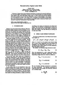
Fig. 1. Typical setup of digital holographic recording of a particle field based on in-line holography.

laser beams, while the developed holograms are brought back to the reference beams to optically reconstruct the 3D images of the particle fields. A CCD camera then scans the 3D image volume mechanically, plane by plane, and the particle field information is computed from the scanned images. A good example is the holographic particle image velocimetry system recently developed by Pu and Meng.5,6 To resolve the spatial structures of a turbulent flow field, millions of tracer particles are seeded in a flow domain to a typical density of 10 –30 particles兾mm3. The silver-halide-based holographic plate, which offers a storage capacity of GBytes 共several thousand line pairs per mm兲, is usually chosen to perform volumetric recording of such large-volume, high-density particle fields. Unfortunately, the holographic plates require chemical developing and fixing, a process increasingly viewed as undesirable by potential users. Furthermore, the optical reconstruction requires tedious 3D mechanical scanning of the reconstructed image volume, a process that takes up most of the data-processing time. This and other HPIV systems involving recording and reconstruction are rather complex and expensive. Consequently, cinematic HPIV7 to provide temporal measurements remains an unfulfilled promise. To circumvent the drawbacks associated with optical holographic recording and reconstruction, over the past few years, digital holography has been explored as an alternative for 3D particle field measurement.8 –10 Figure 1 shows a typical setup for digital particle holography. To minimize the spatial frequency requirement, in-line 共Gabor兲 holography is adopted, where the unscattered part of the illumination wave serves as the reference wave to interfere with the waves scattered by the particles. The interference fringes, whose spatial frequency is proportional to the angle formed by the scattering direction and the reference beam direction, are recorded digitally by a solid-state image sensor and transferred to a computer for numerical reconstruction. The position and size of particles can be obtained from the numerically reconstructed particle field. Particle velocity can also be obtained by measuring particle displacement over two briefly spaced exposures. This approach to digital hologram recording and numerical reconstruction not only eliminates wet chemical processing and mechanical scanning but also enables the use of complex amplitude information that is inaccessible in optical reconstruction. Furthermore, digital holography greatly 828

APPLIED OPTICS 兾 Vol. 42, No. 5 兾 10 February 2003

simplifies the hardware setup for cinematic holographic recording and reconstruction, hence making cinematic implementation of HPIV much easier. Despite these promising prospects, digital holography is inherently limited by the poor resolution of solid-state image sensors. Currently, the pixel size of most scientific CCD sensors is in the range of 6 –10 ␮m, compared with the silver-halide holographic films with an equivalent pixel size down to 0.1 ␮m. Because the digital sensor elements cannot resolve interference fringes finer than the pixel size, the permissible angle between object wave and reference wave is limited to a few degrees. Consequently, the numerical aperture 共N.A.兲 of a digital particle hologram is limited to less than 0.1. The small N.A. leads to a remarkably large depth of focus in the reconstructed particle images. Figure 2 shows the intensity variation along the depth direction in the neighborhood of small particles reconstructed from digital holograms with N.A. ⫽ 0.076. For both 10 ␮m and 20 ␮m particles, the depth of focus based on an 80% threshold is more than 40 times the particle diameter. The large depth of focus results in poor depth resolution and thus severely compromises the 3D capability of digital particle holography. One way to solve the depth resolution problem is to analyze the diffraction patterns in non-image planes instead.11 Several non-image plane methods have been introduced. For example, Onural and Ozgen applied Wigner transform in the recording plane 共holograms兲 to directly compute particle depth positions.12 Ovryn developed a method for predicting particle 3D positions based upon resolving the detailed spatial variations in the scattering pattern.4,13

Fig. 2. Intensity variation near the in-focus position of small particles reconstructed from a digital hologram with N.A. ⫽ 0.076. The depth of focus is approximately 40 times the particle diameter based on 80% threshold.

Vikram and Billet proposed a misfocusing method that utilizes the diffraction patterns in two misfocused planes to extract particle depth position and size.14 Because these methods do not require the knowledge of the exact location of the in-focus planes, they are less sensitive to the large depth of focus of the reconstruction images. A common drawback of these methods, however, is that in the non-image planes the diffraction pattern of individual particles must be segmented first. Consequently, these methods are not practical for measuring a large population of particles, such as those encountered in holographic particle image velocimetry. A new approach, introduced in this paper is to use the complex amplitude of the reconstruction wave that is uniquely available in digital particle holography to extract particles. While optical reconstruction of holograms does not provide convenient access to the complex amplitude of the reconstruction wave 共because sensors used for interrogating the reconstructed 3D image field only respond to intensity兲, in numerical reconstruction the complex amplitude is readily available. Based on digital holographic recording and numerical reconstruction,15 we have developed an automated method for extracting particles from forward-scattering holograms using the complex amplitude of the reconstruction wave. Calibration results have shown that this method significantly improves the depth resolution in digital particle holography as compared with the intensity methods that are often used in traditional optical reconstruction. 2. Real Image Wave at In-Focus Plane

A particle hologram records the complex object wave, O, scattered off small particles through interference with a coherent reference wave. During reconstruction, the same reference wave is diffracted by the hologram either optically or numerically. The resulting reconstruction wave, U, consists of four terms: 共i兲 the real image wave r, which is proportional to the conjugate of the original object wave 共r ⬀ O*兲, 共ii兲 the virtual image wave v ⬀ O, 共iii兲 the directly transmitted wave B, and 共iv兲 the intensity of the original object wave 兩O兩2. Assuming that the real image wave is used in particle extraction, we first study its characteristic near the in-focus plane of a particle. Because Fresnel diffraction is a valid simplification of the Lorenz–Mie theory to predict forward light scattering,16 in what follows we will use the Fresnel diffraction formula to introduce the wave characteristic. Let Aj 共x⬘, y⬘兲 denote the amplitude transmittance function of particle Pj , its scattered wave in the recording plane can be written as o j ⫽ A j 共 x⬘, y⬘兲丢 h zj共␰, ␩兲,

(1)

and zi is the axial distance between the particle and the recording plane. In the hologram reconstruction, the real image wave of particle Pj is obtained from the propagation of the conjugate of the scattered wave, oi *, and can be written as r j 共 x, y, z兲 ⫽ o j * 丢 h z ⫽ A j * 丢 h zj* 丢 h z.

(3)

In the in-focus plane where z ⫽ zj , the convolution between two diffraction kernels in Eq. 共3兲 results in a delta function and thereby rj ⫽ Aj *. In the case of opaque particles the amplitude transmittance function Aj 共or Aj *兲 can be modeled by a real function, therefore the imaginary part of rj vanishes in the in-focus plane of particle Pj . This suggests the possibility of using the imaginary part of the image wave to determine the particle axial position. 3. Dipping Characteristics of Total Reconstruction Field

Ideally, the extraction of reconstructed particle Pj should operate solely on its real image wave rj during hologram reconstruction. However, in reality we cannot separate the real image wave rj from the total reconstruction field U, which also consists of the virtual image wave vj of this particle as well as the wave components associated with other particles. Thus any particle extraction method must operate on the total reconstruction field U. In numerical reconstruction, the directly transmitted wave B, which is the dc component in the frequency domain, can be easily filtered out. Furthermore, the correlation term 兩O兩2 is negligible as compared with other terms in U. What remains in the total reconstruction field in a numerical reconstruction procedure is the superposition of ri and vi of all particles Pi , i ⫽ 1, 2, . . . , N, where N is the total number of particles recorded. To facilitate our discussion, we decompose the total reconstruction field U as U ⫽ rj ⫹ ⍀j ,

(4)

where rj is the real image wave of particle Pj and ⍀j represents all terms in U, which can be written as N

⍀j ⫽

兺 i⫽1

N

vi ⫹

兺

ri .

(5)

i⫽1,i⫽j

We have shown that rj is real in the in-focus plane of particle Pj . However, the imaginary part of U does not vanish due to the addition of ⍀j . Therefore, one cannot directly use Im共U兲 to determine the axial position of particle Pj . To overcome this problem, we examine the variance of Im共U兲,

where R represents convolution, hz共␰, ␩兲 is the Fresnel diffraction kernel

␴ U2 ⫽ ␴ rj2 ⫹ ␴ ⍀j2,

exp共ikz兲 ik 2 h z共␰, ␩兲 ⫽ exp 共␰ ⫹ ␩ 2兲 . i␭z 2z

where ␴2 represents the variance of the imaginary part of the complex amplitude. Here the variance is defined in a transverse plane for all pixels that belong

冋

册

(2)

10 February 2003 兾 Vol. 42, No. 5 兾 APPLIED OPTICS

(6)

829

Fig. 3. 共a兲 Schematic showing the object wave scattered off the particle and the propagate of the real image wave r to the reconstruction planes, 共b兲 variance of Im共r兲 for a single particle computed in the planes near the particle in-focus plane z ⫽ zp. The curve displays the dipping shape with its minimum at the particle depth position.

to the image of particle Pj in that plane. Since the image wave rj is real in the in-focus plane, the variance of its imaginary part, ␴rj2, should be equal to zero in that plane. On the other hand, in other planes aside from the in-focus plane, the imaginary part of rj is not zero and thus its variance is greater. Therefore, the variance of Im共r兲 in the neighborhood of a particle has the minimum on the in-focus plane. We studied the variance of Im共r兲 using computer simulation based on Mie scattering and numerical wave propagation. As illustrated in Fig. 3共a兲, the forward scattered wave off an opaque particle 共dp ⫽ 10 ␮m兲 is obtained by Mie scattering17 in a plane consisting of 512 ⫻ 512 pixels of size 6.8 ␮m. In the second phase, the conjugate of the digitized scattered wave is allowed to propagate 共numerically兲 from the recording plane to different transverse planes at various z positions to obtain the real image wave r. In

each transverse plane, ␴r2 is calculated for all pixels that belong to the particle image in that plane. Figure 3共b兲 shows the variation of ␴r2 with respect to z–zp, the axial distance from the in-focus plane. It is seen in the figure that ␴r2 shows a remarkable dipping shape with its minimum 共⬇ zero兲 at the particle in-focus position. To preserve the dipping shape for an arbitrary particle Pj in the total reconstruction field ␴U2, the change of ␴⍀j2 near the in-focus plane of particle Pj must be negligible as compared to the change of ␴rj2 in the same region. This is verified by comparing the derivatives of ␴rj2 and ␴⍀j2 along the z axis. ⳵共␴r2兲兾⳵z could be simply obtained from the data shown in Fig. 3共b兲, and the result is shown in Fig. 4共a兲. To find ⳵共␴⍀2兲兾⳵z, we simulated a hologram of a densely populated particle field 共number density np ⫽ 12 particle兾mm3兲, and then reconstruct the ho-

Fig. 4. Comparison of the variation of ␴r2 and ␴⍀2 along the axial direction. 共a兲 d␴r2兾dz versus the axial distance from the particle in-focus plane. 共b兲 The cumulative distribution function of 兩d␴⍀2兾dz兩 obtained in the reconstruction of the hologram of a densely populated particle field. Obviously, the axial derivative of ␴⍀2 is much smaller than that of ␴r2 in the neighborhood of the particle. 830


Fig. 5. Experimental demonstration of a digital hologram of 10 ␮m particles on the surface of a glass plate for the purpose of calibration. 共a兲 Hologram fringes recorded on a 12-bit digital camera with pixel size 6.7 ␮m. 共b兲 Numerical reconstructed image at z ⫽ 33.2 mm 共at different planes we obtain different images because the image is three-dimensional兲.

logram on 1,000 consecutive planes with a depth interval equals to the particle diameter. One hundred sample areas in each reconstruction plane were randomly selected to compute ⳵共␴⍀2兲兾⳵z, whose distribution is shown in Fig. 4共b兲. As shown in Fig. 4共a兲, the magnitude of ⳵共␴r2兲兾⳵z is approximately 1.2 ⫻ 10⫺4 at one particle diameter from the in-focus plane, and equals to 1.76 ⫻ 10⫺5 at the in-focus plane z ⫽ zp. These values are much greater than the magnitude of ⳵共␴⍀2兲兾⳵z. Fig. 4共b兲 shows that more than 70% of the samples have 兩⳵共␴⍀2兲兾⳵z兩 less than 1 ⫻ 10⫺5, and more than 95% of the samples less than 5 ⫻ 10⫺5. Therefore, it is very unlikely that the variation of ␴⍀2 will change the dipping shape of ␴r2. As a result, we conclude that the dipping characteristic of real image wave r is preserved in the total reconstruction field U. 4. Particle Extraction Using Complex Amplitude

Using the dipping characteristic preserved in ␴U2, we can identify particles and then extract their depth position. A method called particle extraction using complex amplitude 共PECA兲 was developed based on digital hologram recording and numerical hologram reconstruction. Calibration results and comparisons with intensity-based particle extraction are given in the next section. The steps involved in the PECA method are as follows: 共1兲 Numerically reconstruct the digital holograms on transverse planes at consecutive z positions to obtain the total reconstruction field U on each plane. 共2兲 From the intensity images of U on each scanning plane, label all two-dimensional 共2D兲 objects of bright pixels with gray levels above a threshold value. 共3兲 For each 2D object, find its center position 共x, y兲 and calculate the variance ␴U2.

共4兲 Repeat the process for each scanning plane and construct the 3D objects by clustering the overlapped 2D objects on adjacent planes. 共5兲 For each 3D object, check its record of ␴U2 to see if it has the dipping characteristic. This is to differentiate particles from speckles and other noises in hologram reconstruction. 共6兲 For each 3D object identified as a particle, find the axial position z at which ␴U2 is the minimal through a second-order polynomial regression. The result is saved as the in-focus position of the particle. The radial position of this particle is then copied from the 2D entity that is the closest to the particle’s infocus plane. 5. Results and Discussion

Experimental calibration of the PECA method was carried out using an in-line holography setup as the one shown in Fig. 1. To control the 3D position of particles, polymer microspheres 共10 ␮m diameter, Duke Scientific CAT4210A兲 were placed on the surface of a glass plate that is approximately parallel to the recording plane. The 514.5-nm laser light from an argon laser 共Coherent Innova 90兲 was used for hologram recording. Digital holograms of the particles were directly recorded by a 12-bit CCD camera 共PCO SensiCam兲 with 1280 ⫻ 1024 pixels of size 6.7 ␮m. Figure 5 shows a digital hologram 共after preprocessing兲 and its numerical reconstruction image at z ⫽ 33,200 ␮m 共at different planes we obtain different images because the image is 3D兲. The particle depth positions were extracted from the hologram by use of the PECA method during the numerical reconstruction and plotted against the horizontal position x in Fig. 6. The solid line in the figure represents the glass plate in the x–z plane, which is obtained through the linear regression of particle z–x 10 February 2003 兾 Vol. 42, No. 5 兾 APPLIED OPTICS

831

Table 1. Error in Depth Positions of 10 ␮m Particles Extracted from Digital Holograms

Method

np ⫽ 6 particle兾 mm3

np ⫽ 18 particle兾 mm3

PECA Intensity

6.9 ␮m 29.0 ␮m

12.8 ␮m 41.4 ␮m

Fig. 6. Experimental calibration of the PECA method. Particles originally placed on a glass plate are extracted from the digital hologram shown in Fig. 5共a兲 with the PECA method. The average deviation of the measured distances results 共triangles兲 from the expected locations 共solid line兲 is 22.3 ␮m.

data. This line also indicates the expected positions of particles. It was found that the average deviation of the measurement results from the expected depth positions is 23.1 ␮m 共approximately 2.3 particle diameter兲. The PECA method was further calibrated by the synthesized in-line holograms consisting of 512 ⫻ 512 pixels of size 6.8 ␮m. The holograms record 10 ␮m particles randomly distributed in a 3.5 ⫻ 3.5 ⫻ 10 mm3 volume. Shown in Fig. 7 is a sample hologram with particle number density np ⫽ 18 particle兾mm3. The synthesized holograms were numerically reconstructed and the PECA method was used to extract particle 3D positions from the reconstruction wave field. For comparison, the intensity method, which uses the locations of the intensity peak as in-focus

Fig. 8. Cumulative distribution function of the depth error ␦z obtained by the PECA method at particle concentrations np ⫽ 18 particle兾mm3. The result of the intensity method is also shown for comparison.

positions, was also applied to extract particles from the same holograms. Table 1 summarizes the mean depth error at two particle number densities: 6 and 18 particle兾mm3. It is seen that the PECA method improves the depth accuracy by four folds in each case. The cumulative distribution function of depth error ␦z at np ⫽ 18 particle兾mm3 is given in Fig. 8. With the PECA method, less than 20% of extracted particles have a depth error ␦z greater than 20 ␮m, while with the intensity method more than 70% of the extracted particles have a depth error ␦z greater than 20 ␮m. The great reduction of erroneous particles makes digital holography a more applicable technique to particle dispersion measurement and holographic particle image velocimetry. Calibration of the PECA method based on synthesized holograms with smaller pixel size was also performed. The result shows that the performance of the PECA method further improves as pixel density increases. The PECA method is limited to forward scattering of opaque particles, in which the phase distribution of the scattered wave is symmetric around the optical axis and thus the real image wave shows the dipping characteristic near the in-focus plane. When side scattering or transparent particles are used, the scattered wave has a complicated and irregular phase distribution, and hence the PECA method is no longer applicable. 6. Conclusion

Fig. 7. Synthesized hologram of 10 ␮m particles in a 3.5 ⫻ 3.5 ⫻ 10 mm3 volume with number density of 18 particle兾mm3. 832


Digital holography is a promising technique for 3D measurement of small particles. However, its appli-

cation is often hampered by the poor depth resolution due to insufficient resolving power of the digital image sensors. In this study, we demonstrate that the complex amplitude of the reconstruction field provides a promising solution to this problem. A novel method of particle extraction using complex amplitude 共PECA兲 has been developed for digital holography of a particle field. This method uses the dipping characteristic of the total reconstruction wave to extract the depth position of opaque particles. Calibration results show that the PECA method outperforms the traditional intensity methods and can predict particle 3D position accurately even for densely populated particle fields. With the PECA method, the potential of digital holography could be fully explored in holographic measurement of a particle field as well as holographic particle image velocimetry. This work was supported by a grant from NASA 共NAG3-2470兲 and a grant from National Science Foundation 共CTS-0112514兲.

6.

7.

8.

9.

10.

11. 12.

13.

References 1. A. L. Porta, G. A. Voth, A. M. Crawford, J. Alexander, and E. Bodenschatz, “Fluid particle accelerations in fully developed turbulence,” Nature 409, 1017–1019 共2001兲. 2. M. Virant and T. Dracos, “3D PTV and its application on Lagrangian motion,” Meas. Sci. Technol. 8, 1539 –1552 共1997兲. 3. F. Pereira and M. Gharib, “Defocusing digital particle image velocimetry and the three-dimensional characterization of twophase flows,” Meas. Sci. Technol. 13, 683– 694 共2002兲. 4. B. Ovryn, “Three-dimensional forward scattering particle image velocimetry applied to a microscopic field-of-view,” Exp. Fluids 29, S175–S184 共2000兲. 5. Y. Pu and H. Meng, “An advanced off-axis holographic particle

14.

15. 16.

17.

image velocimetry 共HPIV兲 system,” Exp. Fluids 29, 184 –197 共2000兲. Y. Pu, X. Song, and H. Meng, “Off-axis holographic particle image velocimetry for diagnosing particulate flows,” Exp. Fluids 29, S117–S128 共2000兲. H. Meng and F. Hussain, “Holographic particle velocimetry, a 3D measurement technique for vortex interactions, coherent structures and turbulence,” Fluid Dyn. Res. 8, 33–52 共1991兲. M. Adams, T. Kreis, and W. Ju¨ ptner, “Particle size and position measurement with digital holography,” in Optical Inspection and Micromeasurements II, C. Gorecki, ed., Proc. SPIE 3098, 234 –240 共1997兲. R. B. Owen and A. A. Zozulya, “In-line digital holographic sensor for monitoring and characterizing marine particulates,” Opt. Eng. 39, 2187–2197 共2000兲. S. Murata and S. N. Yasuda, “Potential of digital holography in particle measurement,” Opt. Laser Technol. 32, 567–574 共2000兲. C. S. Vikram, Particle Field Holography 共Cambridge Univ., Cambridge, UK, 1992兲. L. Onural and M. T. Ozgen, “Extraction of three-dimensional object-location information directly from in-line holograms using Wigner analysis,” J. Opt. Soc. of Am. A 9, 252–260 共1992兲. B. Ovryn and S. H. Izen, “Imaging of transparent spheres through a planar interface using a high-numerical-aperture optical microscope,” J. Opt. Soc. of Am. A 17, 1202–1213 共2000兲. C. S. Vikram and M. L. Billet, “Far-field holography at nonimage planes for size analysis of small particles,” Appl. Phys. B 33, 149 –153 共1984兲. L. P. Yaroslavsky and N. S. Merzlyakov, Methods of Digital Holography 共Consultants Bureau, New York, 1980兲. F. Slimani, G. Grehan, G. Goueshet, and D. Allano, “Near-field Lorenz–Mie theory and its application to microholography,” Appl. Opt. 23, 4140 – 4148 共1984兲. P. W. Barber and S. C. Hill, Light Scattering by Particles: Computational Methods 共World Scientific, New York, 1990兲.

10 February 2003 兾 Vol. 42, No. 5 兾 APPLIED OPTICS

833