the Layered Queueing Network (LQN) performance modeling language .... form solution for finding the service times of the parallel branches involved in the join.
1
Deriving Distribution of Thread Service Time in Layered Queueing Networks Tariq Omari, Salem Derisavi, Greg Franks
Department of Systems and Computer Engineering, Carleton University, Ottawa, Ontario, Canada K1S 5B6 {tomari, derisavi, greg}@sce.carleton.ca Abstract— Replication is a technique used in distributed systems to improve performance, availability, and reliability. In replication schemes, often a J out of N voting pattern (also called quorum) is used in which the quorum waits for J replies to arrive. Integrating a quorum scheme into the Layered Queueing Network (LQN) performance modeling language necessitates the computation of the quorum response time as the J th order statistic. To do so, we need the exact (or an accurate estimation of the) time distribution of individual replies. This distribution was estimated in previous work but only for the special case of (J = N ) and yields large errors for J � N . This paper presents a new analytic approach for the derivation of the distributions. Under a number of assumptions, we derive closed form expressions for the probability distribution functions of the replies. The application of our new approach on a number of LQN models shows that, even for models that violate those assumptions, it is far more accurate than previous approaches and it yields an error less than 10% for most example models.Replication is a technique used in distributed systems to improve performance, availability, and reliability. In replication schemes, often a J out of N voting pattern (also called quorum) is used in which the quorum waits for J replies to arrive. Integrating a quorum scheme into the Layered Queueing Network (LQN) performance modeling language necessitates the computation of the quorum response time as the J th order statistic. To do so, we need the exact (or an accurate estimation of the) time distribution of individual replies. This distribution was estimated in previous work but only for the special case of (J = N ) and yields large errors for J � N . This paper presents a new analytic approach for the derivation of the distributions. Under a number of assumptions, we derive closed form expressions for the probability distribution functions of the replies. The application of our new approach on a number of LQN models shows that, even for models that violate those assumptions, it is far more accurate than previous approaches and it yields an error less than 10% for most example models.
I. INTRODUCTION Replication is a technique used in distributed systems today to achieve high performance, high availability, and fault tolerance. Replication maintains copies of data and services in multiple locations and allows requests to access any one of the copies. It improves performance by reducing the distance
between an application and the data it has to access, by having multiple sites from which can spread the load, or by bringing the aggregate of the computing power of all the replicated sites to bear on a single load category. For example, Google uses replication for better request throughput [1]. Other practical examples include web databases [2] and grid computing. Replication improves availability and reliability by letting applications use any copy of the data. For example, replication is used in a peer-to-peer content distribution [3] for improving the availability of content, enhancing performance, and resisting censorship attempts [4]. Replication is used for fault tolerant design with Redundant Arrays of Inexpensive Disks (RAID) [5] and in safety critical systems like air traffic control [6]. There are two fundamental approaches of replication for improving reliability and availability. The first is modular redundancy in which each component performs the same function [7], [8]. The replicas here are called active or static replicas. The second approach involves primary/standby schemes, in which when a primary component is functioning normally it periodically sends its state to the secondary replicas. The secondary replicas remain on stand-by and takes over if the primary fails. These replicas are called passive or dynamic replicas. One example of active redundancy is Triple Modular Redundancy (TMR), which is a special case of the generalized NMR (N-Modular Redundancy), where the effect of a fault is masked instantly. In TMR, there are three identical processing modules and majority voting is performed on the output of the modules to select the final output result. A. A Quorum Pattern In a quorum pattern, a client selects a quorum or a certain number of replicas to update or read. An operation is allowed to proceed to completion when a subset of nodes responds to requests made by that operation. For example, in Fig. 1 after the client sends three requests to three independent replicas; it waits only for the first two responses. The quorum is preset to two, meaning the client needs to wait only for two replies from the replicas in this case. After the client receives the two replies it resumes execution. All other replies that are received after the quorum is done are ignored in this pattern. Different semantics based on other patterns are also possible. In Fig. 1, the last reply (message number 6) that occurs after the quorum action is ignored; it does not affect the performance. When the quorum is set to one, then this pattern handles the cases in which only the first response is needed as is the case
2
Client
Replica1
Replica2
Replica3
User 1
User 2
User n
[1]Read [2]Read Parallel
[3]Read
Application
[4]Reply [5]Reply [6]Reply
Fig. 1.
A quorum pattern.
in broadcasting. When the quorum is set to the number of replicas, then this is a voting example where all the responses are needed. In quorum consensus (QC), or voting, protocols, an operation can be allowed to proceed to completion if it can get permission from a group of nodes. The weighted majority QC algorithm [9], generalizes the notion of uniform voting. Instead of assigning a single vote per site, each copy ds of a data item d is assigned a non negative weight (a certain number votes) whose sum over all copies is u. In general, quorum consensus methods [10], allow writes to be recorded only at a subset (a write quorum) of the up sites. This is given that reads are made to query a subset (a read quorum) that is guaranteed to overlap the write quorum. This quorum intersection will ensure that every read operation will be able to return the most recently written value. Voting termination requires an extra round of messages to coordinate the different replicas. This round can be as complex as an atomic commitment protocol (for example, the two-phase commitment protocol), or as simple as a single confirmation message sent by a given site. The main drawback of quorum consensus protocols is the relatively high overhead incurred in the execution of the read operations. B. Performance Modeling Whether the system was designed for performance, reliability, or availability purposes, the system can be modeled and solved for performance. The quorum is used for those models which require to wait for a consensus of the responses before the main thread of control can resume execution. The quorum pattern above presents interesting problems for creating analytic performance models because the quorum-join amounts to finding the distribution of the completion, or service, time of the j th response of the N replica branches. The quorumjoin time is very sensitive to the distribution functions of the N branches. Previous methods for finding these distributions include the “three-point” approximation [11] and the gamma distribution [12]. If a client makes a deterministic number of calls to the server, the results show that gamma distribution works well. However, if the client makes a random number of calls with a geometric distribution, the errors are much worse.
Fig. 2.
DataBase1
DataBase2
Disk1
Disk2
DataBase3 Disk3
Disk4
Replicated database.
C. Contributions The contributions of this paper are summarized as follows: 1) Deriving a closed-form formula for the cumulative distribution function, cdf, for a thread service time when the calls that the thread makes are geometrically distributed. 2) Deriving a closed-form formula for the probability density function, pdf, for a thread service time when deterministic calls are used. This is used to justify the usage of gamma distribution fitting as it is a special case. 3) Showing that the three-point distribution and the gamma distribution are inadequate for fitting threads with geometric calls. 4) Showing that a gamma distribution is a good estimate for the thread’s service time when deterministic calls are used. The results obtained from test runs show that the new formula works much better than the three-point approximation and gamma distribution. Our results were verified by comparing them to simulations and to the solutions of Markov chains generated from PetriNet models with quorum. The remainder of the paper is organized as follows. Section II describes the framework for the modeling effort, Layered Queueing Networks. Section III describes the new closedform solution for finding the service times of the parallel branches involved in the join. Section IV shows how the new approximation compares to the other approximations and simulation and exact analytical results. Finally, Section V gives our conclusions. II. LAYERED QUEUEING NETWORK MODELS A Layered Queueing Network (LQN) is a form of extended queueing network designed to model software systems with nested resource requests as is commonly found in a multi-tier client-server systems. Layering arises when a client makes a request to an intermediate server (for example, the Application server shown in Fig. 2), who in turn makes requests to servers at even lower levels. While a lower-level server is processing a request, all of the intermediate servers between this server and the client are blocked. This type of interaction is a form of simultaneous resource possession where the order of acquisition and release is strictly hierarchical.
3
Fig. 3 illustrates the notation of an LQN using the example shown earlier in Fig. 2. The large parallelograms denote “tasks” which can represent customers in the network, software servers, logical resources, and hardware devices. Tasks can make requests to other tasks, and always have an associated processor. Tasks can have a multiplicity, denoted by the stacked task icon and the label in braces, representing multiple homogeneous copies of the task. Tasks which only make requests to other tasks represent customers in the network; here the multiplicity represents the number of customers. For all other tasks, the multiplicity represents the number of identical servers servicing a single queue of requests. The circle icons in the figure represent the “processors” in the model. Processors serve to consume time for activities and may represent actual hardware processors as is the case with the application and three db tasks or simply serve as a place holder as is the case with the task client. The association between a task and its processor is shown with the unlabeled arc to the processor icon although if there is a one-to-one relationship the processor is often not shown. Processors may also have a multiplicity, again shown as a stacked icon. If the multiplicity of the processor is “infinity”, then the processor is simply a delay server. The small parallelograms found inside the task icons are called “entries” and serve as interfaces for different classes of service provided by the task (tasks may have several entries, though this is not shown here). The details of an entry are specified through either “phases”, or by a sequence of “activities”, shown as small rectangles with predecessor-successor relationships, with a first activity in the graph triggered by the entry. Service times for activities and entries are shown on the figure using labels with square brackets. In Fig. 3, the entry application triggers the execution of the activity recv followed by the activities send1, send2 and send3 all executing concurrently, and ending with the activity reply. At the end of activity reply, a reply is sent by the entry application to the client’s entry client, and the service is over. This particular graph illustrates an AND-fork and join. The notation also supports choice and looping constructs, so that task graphs such as those used by Smith [13], can be represented directly. Service requests are always made from activities or phases to entries. Two types of requests exist: • a synchronous or blocking remote procedure call (RPC), indicated in Fig. 3 by solid arrows with closed arrowheads. Clients making this type of request are blocked until they receive a reply. Replies are typically sent to the task originating the request. Alternatively, the reply may be forwarded to another entry for a later reply • an asynchronous request. Clients making this type of request continue in parallel with their server; no reply is expected. Neither the forwarded reply nor the asynchronous request types are used in Fig. 3. Mean number of requests to entries are shown in Fig. 3 using labels with parenthesis. If the request originates from an entry using the simplified notation, a list will be shown with each item corresponding to a phase from the originating entry.
Number of requests can be either distributed geometrically with the given mean value, or deterministically. For the former case, the geometric random variable takes non-negative integer values by definition. For the latter case, the number of requests must be set to a non-negative integer as well. These requests are tagged with the letter ‘D’, for example, the arc from send1 to db1 in Fig. 3. A. Solving Layered Queuing Network Models In software systems, delays and congestion are heavily influenced by synchronous interactions such as remote procedure calls (RPCs) or rendezvous. Fig. 3 shows the tasks and processors in a model arranged in layers, sorted with requests originating from a higher layer entity and being made to a lower layer one (note that requests may jump over layers and, in the general case, can also go up to a higher layer). The LQN model captures these delays by incorporating the lower layer queueing and service times into the service time of the upper layer server, i.e., an entry’s service time is not constant but is determined by its lower servers. Thus the essence of layered queueing is a form of simultaneous resource possession because a customer “holds” both the client and the server during the duration of a rendezvous. This “active server” feature [14] is the key difference between layered and ordinary queueing networks. The overall LQN model is solved by first constructing a set of submodels consisting of a set of clients and a set of servers. The analytic layered queueing network solver, LQNS, used in this research, constructs these submodels by finding all of the serving tasks and processors at a given layer L > 1, and treating these as queueing stations, then finding all the clients who call these servers at any layer except L, and treating these as customers [15]. Each client in the submodel forms a unique routing chain in the queuing network model. For example, Fig. 4(a) shows the components that make up the first submodel for the LQN model shown in Fig. 3; the corresponding queueing network is shown in Fig. 4(b). Each of these submodels is then solved using either BardSchweitzer [16], [17] or Linearizer [18], [19] approximate Mean Value Analysis (MVA) [20]. The residence times found as an output for a particular submodel are then used to find the service times for inputs to other submodels using the method of surrogate delays [21]. Other approaches to solving layered queueing networks include the Method of Layers [22], Stochastic Rendezvous Networks [14], and others [23], [24], [25], [26]. B. Modeling Tasks with Internal Parallelism Parallelism arises in Layered Queueing Networks through the use of asynchronous messages, early replies from serving tasks, and through internal parallelism within a task1 through the fork and join pattern shown earlier in Fig. 3. Only the latter form of parallelism is described here and it has the following execution semantics. Each task, with the exception of the pureclient tasks2 , consists of a single principle thread of control 1 Internal parallelism within a task is not the same as having multiple copies of the same task. 2 Pure client tasks do not accept messages.
4
client [10]
Layer 1
client {4} (1) application
client {inf}
application recv [0.1] & send1 [0.001]
Layer 2
send2 [0.001]
send3 [0.001]
& reply [0.1] client
application
(1D)
(1D)
db1 [1]
db2 [1]
db3 [1]
db1
db2
db3
db1
db2
db3
(1D) Layer 3
application
db[1−3]
Synchronous request
Fig. 3.
Layered queueing network of the example system in Fig. 2.
client [10]
client {4} client [0]
client {4} (1)
client {inf}
application [0.203]
client (2)
client:application (1)
application
client {inf} client [5]
application application [0.203]
Submodel 1
(a) Submodel components. Fig. 4.
Layer 4
(b) Queueing model.
Submodel 1 from Fig. 3.
which continually loops waiting for messages, then processes the corresponding requests when one arrives. The behavior of a task with internal parallelism is more complicated. When the main thread of control for the task reaches the fork point, denoted by the circle labeled with an ampersand in Fig. 3, independent threads of control are created, one for each branch after the fork point. These threads of control continue until they reach the join point, also denoted by a circle labeled with an ampersand in the figure, whereupon they are destroyed. Once all of these threads have completed, the main thread of control continues. Note that this behavior itself may nest, where the sub-threads also may fork new threads which then later join. Two problems arise when trying to solve product-form queueing models with fork-join behavior: 1) creation of customers in the queueing network through the fork, and 2)
computation of the synchronization delay. The creation of customers in the queueing network is a problem because this action violates the conditions of product-form solution. A common approximation creates separate routing chains for each of the threads in the model [27]. The time needed for all of the sub-threads to complete execution, i.e. the join delay, is inserted as a surrogate delay into the service time of the parent thread. Mak and Lundstrom [28] improved upon this technique by removing contention between the parent and child threads in the queueing model. This approach is further generalized to multi-servers in [29]. The second problem for solving queueing networks with fork-join behavior is the computation of the synchronization delay itself. The AND-join delay is found by taking the product of the distributions of the execution times of all of branches involved. In general, these distributions are not known a-prior, so some distribution is assumed, typically exponential. In a layered queueing network, the execution time distribution of an activity is typically not exponential because activities make blocking requests to lower level servers. (This is the subject of the current research and is described in greater detail below.) These blocking requests cause the execution of the activity to be broken up into a possibly random number of slices, with the slices themselves having non-exponential service time distributions. Further, when solving the model analytically, Mean Value Analysis does not compute higherorder moments so only the mean time to lower-level servers is known. An auxiliary model must be solved, though it only
5 Probabilites aj
A(t)
0.54
1.0
0.42 1−a3=0.58 a1=0.04
0.04 t1
t2
(1.37) (2)
t
t
t3
t1
t2
(1.37) (2)
(3.26)
t3 (3.26)
(a) Probablity mass function. (b) Probability distribution function. Fig. 5.
Three-point distribution with mean=2.0 and variance=0.4.
supplies variance [12], [22], [14]. Notwithstanding these limitations, a simple “three-point” approximation was found to be effective for computing ANDjoin delays where a discrete distribution was fit to the mean and variance using only three points [11]. Fig. 5 illustrates the point probabilities aj (t) for one thread and the approximation A(t) for the probability distribution function for that thread. The locations tj , for j = 1, 2, 3, of the three points and the values aj for their probabilities are derived from the mean, µt , and variance, σt2 , of a service time as follows: step 1: Find the locations for the three points ( µt − σt µt − σt > 0 t1 = 0 otherwise t2 = µt t3 = µt + 2kσt where k = max{1, µσtt }. step 2: The discrete probabilities aj at the special points tj are calculated so as to give a discrete distribution with the same mean and variance, used in step 1, as follows: 3 X
tj aj
= µt
t2j aj
=
µ2t
=
1
j=1 3 X
paths in the quorum-join is found by calculating the J th order statistic [31] for the delays of all of the branches. For an AND fork-join, J = N , which is the maximum of the branch times. To find the J th order statistic, a probability distribution function is needed for each branch service time, not just the mean and variance. In [29], the three-point method described above was used, with good results. In [12], a gamma distribution was used for fitting the thread service time distribution for estimating soft deadlines. In both of these cases, the tails of the cumulative distribution functions were more important in calculating the result than any other part of the distribution. The last aspect of the calculation is treatment of the extra routing chains added to the MVA submodel to accommodate the fork. In a quorum join, the main thread of control (the parent) is forked into N child threads and then pauses execution. Next, when any J out of the N threads respond, the main thread resumes. However, there are now (N − J) “surplus” threads which were not part of the join that must be dealt with. Two different possibilities exist: 1) the surplus threads can all be aborted, although this action may be difficult to accomplish in practice, as the surplus threads may be blocked on lower level servers, which in turn will have to be aborted. 2) the threads may continue to execute, with the parent thread ignoring their results. If the parent thread finishes and accepts new requests while the surplus threads are still executing, there is a possibility of exhausting resources as surplus threads may continue to build up in the system. Alternatively, the parent thread may wait until all of its child threads complete, i.e., an implicit join at the end of the parent thread. This work is only concerned with the estimation of the quorum delay itself, so the semantics of the disposition of the surplus threads is beyond the scope of this paper. III. SOLUTION OF LQN WITH QUORUM
+
σt2
j=1 3 X
aj
j=1
The choice of the points tj was important for the accuracy of the approximation [11]. The likely reason for this success of this approach when used in an AND fork-join pattern is that the maximum of several distributions is weighted to the tails. C. Quorum in LQN The solution of a model with a quorum join is a more general case of solving a model with internal parallelism. First, submodels are solved using Mean Value Analysis to find the average residence time at each queueing station. Second, an auxiliary model [12] is solved to find the variance for each activity. Next, sequences of activities which do not involve forks and joins are aggregated into a single activity using the technique in [30]. Finally, the overall delay for J out of N
In a Layered Queueing Network model, a client can make a sequence of synchronous calls to a server. The number of calls can be deterministic or geometrically distributed. According to LQN semantics [32], upon accepting a new customer, the client enters in a cycle during which it alternates service periods of its own with requests made to other servers for nested calls. By default, the client’s own service periods are random with an exponential distribution with a mean that is fixed across the different synchronous calls and it is stateindependent. A service time with a coefficient of variation different than one and greater than zero can be specified in the LQN input model, but this is not handled in this paper. Note that the distribution of the service time of each call is not necessarily exponential because the server itself may call other servers. In the numerical solution of LQN using MVA, it is important that we compute the distribution of the total service time of a client’s own service time and all its calls as accurately as possible. That is needed to compute the distribution (and therefore, the mean and variance) of the service time of a quorum construct using the J th order statistic formula in [31]
6
for independent random variables. In order to compute the J th order statistic, the cumulative distribution function for each random variable has to be determined. The random variable here is the total service time of a client, or a thread, calling server(s). Previously, the three-point distribution was used to approximate the distribution of the service time of a thread. It was then used to compute the mean and variance of the service time of an And Join using a special case of J th order statistics formula (J = N ). Since the errors in the final results were tolerable we concluded that And Join formula is not very sensitive to variations in the input distribution as long as they match the correct distribution in the first and second moments. However, based on our experiments (shown in Section IV), we found out that using three-point distribution as input in J th order statistics formula (for quorums) generates unreasonable error. That motivated us to propose more formal approaches for the derivation of the distribution of the thread service time. In order to make the derivation possible, we temporarily restrict our discussion to models for which the following conditions hold: 1) The client calls only one server. 2) The distribution of the call’s service time is exponential. This holds only if the server does not call any lower layer servers. 3) After the MVA solution of a submodel, which accounts for contention in shared resources between threads, the threads’ service times are assumed to be independent. In section IV, we will show that except for a few test cases, the final results that we compute based on the distributions derived in this section, have errors less that 10% even for models that do not conform to the conditions above. In the rest of the section, we first express the problem in mathematical terms and introduce our notation. Then, we derive the distribution of the thread service time depending on whether the number of calls to the server is deterministic or geometrically distributed. Finally, we summarize our findings.
As we previously mentioned, LQN syntax allows the distribution of K to be either geometric or deterministic. So we will consider two cases: when Kis geometrically distributed, and when K is deterministic.
B. K is Geometrically Distributed When K’s distribution is geometric we derive an exact closed-form expression for fZ and FZ . In order to do so, we transform the functions into the frequency domain using Laplace transform without which the derivation would involve modified Bessel functions [33], and therefore, more difficult to R +∞ manipulate. We use L{fX }(s) = 0 e−st fX (t)dt to denote the Laplace transform of fX (t). Note that the steps of the derivations in the rest of this section, including the Laplace and inverse Laplace transforms, are all performed symbolically (as opposed to numerically). Only the final result (FZ ) will be evaluated numerically during the numerical solution of the LQN. Let the probability mass function of K be Pr{K = k} = p(1 − p)k where k ∈ {0, 1, . . .} and 0 < p ≤ 1. Note that E[K] = p1 − 1, and hence, p can be calculated given the mean number of calls that the modeler provides in the LQN model specification. Moreover, when K is geometric E[K] does not need to be an integer. We consider two cases: E[Xc ] = 1/λc 6= 0 and E[Xc ] = 0.3 E[Xc ] = 0 arises if the client spends zero (or a negligible amount of) time at its own processor. The reason we consider it as a different case is that λc is not a real number and cannot be plugged in the final result. 1) Case E[X Pk c ] 6= 0: Let the random variables PK W = Xc + Xs , Wk = W (k ≥ 0), and W = K i=1 i=1 W . Since fXc (t) = λc e−λc t and fXs (t) = λs e−λs t , we have
A. Notation and Formal Problem Description The problem is to compute the distribution of the thread service time, i.e., the time it takes for a client to complete all its internal processing and all its calls to the server. Let X be an arbitrary random variable (RV). We use fX , FX , and E[X] to denote the pdf (probability density function), the cdf (cumulative distribution function), and the expected value of X respectively. Let Xc be the exponential RV with rate λc associated with service time of each internal processing of the client c, and Xs be the RV associated with the service time of each call to the server s. Based on above conditions, Xs is exponentially distributed with a given rate λs . We have fXc (t) = λc e−λc t fXs (t) = λs e−λs t
L{fW } = L{fXc } · L{fXs } =
λs λc · s + λc s + λs
Moreover,
L{fWk } = fWK (t)
=
(L{fW })k = ( ∞ X
λc λs )k (s + λc )(s + λs )
fWk (t) Pr{K = k}.
(1)
k=0
FXc (t) = 1 − e−λc t E[Xc ] = θc = 1/λc FXs (t) = 1 − e−λs t E[Xs ] = θs = 1/λs Taking the Laplace transform of both sides of Eq. 1, we will have: PK The RV Z = Xc + i=1 (Xc + Xs ) gives the total service time where K is a non-negative integer random variable associated with the number of calls. We are, in fact, interested 3 E[X ] cannot be zero because it would be meaningless to call a server s with zero service time. So E[Xs ] 6= 0 always holds. in computing FZ .
7
PK
i=1
L{fWK (t)} = = =
∞ X k=0 ∞ X k=0 ∞ X
L{fWk (t)} Pr{K = k}
k=0
=
=
(
λs k ) (1 − p)k p s + λs
= p
k=0
λc λs (1 − p) k ( ) (s + λc )(s + λs )
= p
1 1−
k=0 ∞ X
k=0 ∞ X
λc λs )k (1 − p)k p ( (s + λc )(s + λs )
= p
= p
L{fZ (t)} = L{fWK (t)} ∞ X = L{fWk (t)} P r{K = k}
L{fWK (t)|K = k} Pr{K = k}
k=0 ∞ X
Xs . Therefore,
λc λs (1−p) (s+λc )(s+λs )
p(s + λc )(s + λs ) (s + λc )(s + λs ) − λc λs (1 − p)
(2)
Moreover, using Z = Xc + WK and Eq. (2), we continue:
(
λs (1 − p) k ) s + λs 1
1−
λs (1−p) (s+λs )
p(s + λs ) λs p(1 − p) = =p+ (5) s + λs p s + λs p Taking the inverse Laplace transform of Eq. (5), we have fZ (t) = pδ(t) + λs p(1 − p)e−λs pt for t ≥ 0. Hence, ( 0 t=0 (6) FZ (t) = −λs pt p + (1 − p)(1 − e ) t>0 C. K is Deterministic
L{fZ } = L{fXc } · L{fWK } p(s + λc )(s + λs ) λc · = s + λc (s + λc )(s + λs ) − λc λs (1 − p) pλc (s + λs ) = (3) (s + λc )(s + λs ) − λc λs (1 − p) To derive fZ , we need to use the partial fraction decomposition method, that is, to find A1 and A2 such that A1 A2 L{fz } = s+γ + s+γ where −γ1 and −γ2 are the roots of 1 2 the denominator of L{fZ }. Performing the calculations yields
γ1
=
γ2
=
A1
=
A2
=
p (λc + λs )2 − 4pλc λs p 2 λc + λs − (λc + λs )2 − 4pλc λs 2 pλc (λs − γ1 ) (γ2 − γ1 ) pλc (γ2 − λs ) (γ2 − γ1 ) λ c + λs +
x
FX (x) = 1 − e− θ
Using the inverse Laplace transform, fZ (t) = A1 e−γ1 t + A2 e−γ2 t , and by integration FZ (t) = 1 − (A1 /γ1 )e−γ1 t − (A2 /γ2 )e−γ2 t
When K is deterministic, we assume that E[K] = k ∈ N4 . In this case, we are able to derive the closed form of fZ but R we cannot derive FZ (t) = fZ (t)dt in closed form for all cases. Before we derive fZ , we introduce two distributions: Gamma and McKay. Definition 1: A continuous RV X follows the gamma distribution with shape i > 0 and scale θ > 0 when its probability density function can be expressed as follows: ( 0 x −(1/2), b > 0, |c| < 1 when its probability density function can be expressed as follows: ( 0 x θs , and θc < θs . 4 Because it is meaningless to call a server a non-integer or negative number of times.
8
1) Case P θc = θs : Let θc =Pθs = θ, then Xc = Xs and 2k+1 k Z = Xc + i=1 (Xc + Xs ) = i=1 Xc . Therefore, Z has a gamma distribution with shape 2k + 1 and scale θ. Using Eq. (7), its cdf can be written as: ( 0 t≤0 (8) FZ (t) = P2k i 1 − e−t/θ i=0 θti i! t > 0 Pk Now consider Z = Xc + i=1 (Xc + Xs ) = Xc + Pk Pk Xc + i=1 Xs where k = E[K] and θc 6= θs . Yc = Pi=1 k i=1 Xc is the sum of k exponential RVs with mean θc . Therefore, Yc has a gamma distribution with parameters k and Pk θc . Similarly, Ys = i=1 Xs has a gamma distribution with parameters k and θs = 1/λs . It can be shown (e.g., see [35]) that the the RV Y = Yc + Ys has a McKay distribution with parameters a=k−
1 2
2θc θs |θc − θs |
b=
c=
θc + θs . |θc − θs |
Since Z = Y + Xc and the pdf of sum of two RVs is the convolution of the pdfs of the RVs, functions we have: Z t fZ (t) = fY (x)fXc (t − x) dx 0 √ 2 Z t t−x c π(c − 1)a+1/2 x = xa e− b x Ia ( )e− θc dx 2a ba+1 Γ(a + 1/2)θc 0 b | {z } − θtc
Z
D t
= De
0
c 1 x xa e−( b − θc )x Ia ( ) dx b
(9)
There are two subcases: θc > θs and θc < θs . c −θs 2) Case θc > θs : We have cb − θ1c = θ2θ = 1b . Using c θs formula 11.3.12 of [34], variable change of z = x/b, and a number of simplification steps we derive the following equality: t Z t ta+1 e− b (Ia ( bt ) + Ia+1 ( bt )) x x . (10) xa e− b Ia ( ) dx = b 2a + 1 0 Continuing Eq. (9), we have fZ (t)
ta+1 (Ia ( bt ) + Ia+1 ( bt )) 2a + 1 c De−t b ta+1 (Ia ( bt ) + Ia+1 ( bt )) 2a + 1 1
1
= De−t( θc + b ) =
since 1b + θ1c = cb . c −θs 3) Case θc < θs : In this case, cb − θ1c = θ2θ = − 1b . c θs Similar to Eq. (10), we can derive the following equality:
We conclude that −t c De b ta+1 (Ia ( bt )+Ia+1 ( bt )) 2a+1 c fZ (t) = De−t b ta+1 (Ia ( bt )−Ia+1 ( bt )) 2a+1
θc > θs
(12)
θc < θs
If θc = θs , Eq. (8) gives FZ . However, when θc 6= θs , we do not know how to derive the indefinite integral of Eq. (12) and derive FZ (t) in closed form. We are currently investigating the matter. D. Violation of the Conditions The closed-form formulas that we developed above were derived using a number of assumptions we mentioned in the beginning of the section. Now, we explain the approximation approaches we take in using those formulas when the first two assumptions are violated. In Section IV, we evaluate the effect of the approximations. 1) Calling More than One Server: The first assumption is that a client thread calls only one server. Otherwise, a thread calls a set of servers s1 , . . . , sj (j > 1). According to LQN definition, the distribution of the number of calls to the servers has to be the same for all servers (i.e., either all geometric or all deterministic). In this case, we use an approximation method and replace the set of servers by a single server. Let θsi be the mean service time of server i, ki be the average number of calls from the client to server i (1 ≤ i ≤ j), θs be the mean service time of the approximated server, and k be the average number of calls from the client to the approximated server. Our approximation computes k and θs such that it conserves the average number of calls and also the mean of the total service time. More formally, k=
j X i=1
ki
j 1X θs ki . θs = k i=1 i
(13)
2) Non-exponential Service Times: The second assumption is that the server has an exponentially-distributed service time. This is a valid assumption if the server does not make lower layer calls. However, if the server makes lower layer calls the service time of the server will not be exponentially distributed and, to the best of our knowledge there will be no closed-form formula for the thread service time. In this case, we simply approximate the (non-exponential) distribution of the service time with an exponential distribution that has the same mean as that of the non-exponential distribution. E. Summary
t
Z 0
t x x xa e b Ia ( ) dx = b
a+1
e
t b
(Ia ( bt )
− 2a + 1
Ia+1 ( bt ))
.
Continuing Eq. (9), we have fZ (t)
= since
1 θc
−
ta+1 (Ia ( bt ) − Ia+1 ( bt )) 2a + 1 c De−t b ta+1 (Ia ( bt ) − Ia+1 ( bt )) 2a + 1 1
1
= De−t( θc − b )
1 b
= cb .
(11)
In this section, we derived closed form formula for FZ when K, the number of calls to the server, is geometrically distributed (See Eqs. (4) and (6)). It means that provided that the assumptions hold, we can exactly compute the distribution of the quorum join delay. When K is deterministic and θc = θs , we found out that Z has a gamma distribution and we also derived a closed form for FZ (See Eq. (8)). However, for the case of θc 6= θs , we could derive fZ but not FZ . The problem is that the J th order statistics formula
9
in [31] uses fZ and not FZ . That leaves us with two choices: 1) to use numerical integration of fZ to evaluate FZ , or 2) to approximate FZ with a distribution that has a closed form. The results shown in Section IV are not based on numerical integration of fZ . Instead, we have temporarily selected the second choice above. In particular, we have approximated FZ with a gamma distribution that has the same mean and variance as those of FZ . The reason we choose gamma distribution is that FZ follows that distribution when θc = θs (See Eq. (8)). We will show in the next section that this approximation performs fairly well although it seems to be a rough approximation. IV. RESULTS AND ANALYSIS In this section, the accuracy of fitting the distribution of a thread service time to the new derived closed-form formula, a gamma distribution, or a three-point distribution is evaluated. We consider three LQN models, each of which with several configurations. For each configuration, the quorum join delay is computed using three methods: (1) LQNS using different distributions, (2) simulation, and (3) exact solution of the Markov chain of the model (if possible). LQSim, the simulator module for LQN models, has been modified to simulate the LQN model with a quorum fork-join. The Markov chain is generated from a PetriNet model of a LQN model with a quorum and is solved using GreatSPN. The results from the three methods are compared. As mentioned in Section III, we derived the distribution of the thread service time assuming that a number of conditions hold. Different LQN models are presented to show the accuracy of the distributions both when those assumptions are satisfied and also when they are violated. In particular, in Sections IV-B and IV-C, we study two LQN models for which the first and the second assumptions do not hold, respectively. For each model, we examine the results for when the average number of calls to lower layer servers is deterministic or geometrically distributed. Moreover, various combinations of parameter values are chosen to see whether the errors, in the approaches we study, are sensitive to the different parameters involved. Particularly, we have varied the ratio of the client’s service time to the server’s service time from a low to a high value. A. Effect on a One-Layer Model Fig. 6 shows an LQN model with task B1 having 6 threads. When a customer arrives to entry B1, the main (or first) thread of the task is started, invoking entry B1 which calls activity aa in turn. When activity aa completes execution, the main thread forks into five threads: threads 1, 2, 3, 4, 5 that execute activities a1, . . . , a5 respectively. The execution of each of these five activities requires calls to the lower layer servers C1, . . . , C5 respectively. Activities ai, ∀i = 1, . . . , 5, each has an execution demand of A time units, and entries Ci each has an execution demand of C time units. The circle with “q(1)” notation inside it means that the main thread will resume execution after the fork if any one of the five forked threads respond (J = 1). After the quorum takes place, the
B1
B1
aa [1] & a1 [A]
a2 [A]
a3 [A]
a4 [A]
a5 [A]
q(1)
Reply [10]
(y)
(y)
(y)
(y)
(y)
C1 [C]
C2 [C]
C3 [C]
C4 [C]
C5 [C]
C1
C2
C3
C4
C5
Fig. 6.
One-layer LQN model with a quorum notation.
main thread will resume execution and it will execute activity Reply. Our objective here is to analytically calculate the time required since forking the main thread until we receive one out of the 5 threads: this time is the quorum join delay. Table I shows the quorum join delay for the LQN model of Fig. 6 when all calls, shown as the parameter y, from forked threads to the servers are deterministic. The tuple in the first column of the table is the average number of deterministic calls by a thread to a server, the execution demand (A) of activities ai, and the average execution demand (C) for entries Ci for i = 1, . . . , 5. The second column is the exact solution for the time delay of the quorum join calculated from a Markov chain generated from a PetriNet model of the LQN network. This solution does not compute the variance. The third column shows the mean and variance result from simulating the LQN model using LQSim. The simulation confidence intervals of ±95% for all values of the mean are less than 5%, and for the variance are less than 10%. The results from the Markov chain solution show that the simulation results were highly accurate. The remaining columns show the relative error of the analytic solution computed using LQNS using the three-point approximation and the gamma distribution fitting compared to the simulation results. This error is found by dividing the difference of the simulation and analytic results by the simulation result, and multiplying by 100. The results show that the gamma distribution is the best fit with an absolute error of less than 2% for the mean join delay. Table II shows the quorum join delay for the LQN model of Fig. 6 when the threads makes two geometrically distributed calls (parameter “y” in the table) to the lower layer servers Ci. This model is solved using Markov chain for an exact solution, simulation, and analytically using LQNS. For the analytic solutions, three distribution fittings are used: the threepoint approximation, the gamma distribution, and the closedform formula for geometric calls. As is shown in the table, the relative error in the mean for the quorum join delay can go up to about 34% for the case of three-point approximation, and up to 70% for the gamma fitting, while using the closed-form formula the errors are less than 10%.
10
TABLE I Q UORUM
JOIN DELAY OF THE ONE - LAYER MODEL WITH DETERMINISTIC CALLS IN
Parameters (y,A,C)
Markov Chain mean 4.4623 7.5956 3.7579
(2D,1,5) (2D,5,5) (2D,5,1)
LQSim mean 4.4541 7.6007 3.7562
variance 4.9122 8.2053 1.782
LQNS Three-point mean variance 8.70% 18.15% 10.12% -18.02% 12.07% -33.14%
F IG . 6.
Error Gamma mean variance -1.29% 10.12% -1.29% 8.22% 0.83% -0.48%
TABLE II Q UORUM Parameters (y,A,C) (2,1, 5) (2,5, 5) (2,5,1)
JOIN DELAY OF THE ONE - LAYER MODEL WITH GEOMETRIC CALLS IN
Markov Chain mean 0.67976 1.7245 1.2496
LQSim mean 0.67802 1.7238 1.2438
variance 2.7914 6.5239 1.8738
Three-point mean variance 34.28% 230.14% -14.53% 206.85% -30.43% 185.07%
F IG . 6.
LQNS Error Gamma mean variance 70.23% 1.49% 21.77% 3.59% 8.52% -2.61%
Closed-form-geo mean variance 9.10% 0.62% 5.68% 0.03% 3.69% 0.39%
B. Effect on a One-Layer with a Multi-Call Model In this section, the accuracy of different distribution fittings is evaluated when a thread makes calls to more than one server. This case violates the assumptions made for the closedform formula for geometric calls because the service times at the server are likely different. Fig. 7 shows the model used, with each forked thread i calling two lower layer servers Ci1 and Ci2 for i = 1, . . . , 5. The number of calls to entries Ci1 and Ci2 are represented by the variables y1 and y2 respectively. The variables Cx1 and Cx2 represent the execution demands at the server. The accuracy of the various distribution approximations for both geometric and deterministic calls are shown in Tables IV and III respectively. Table III shows the result of fitting the thread service times to a three-point and a gamma distribution when the calls y1 and y2 in Fig. 7 are deterministic when 1 out of 5 forked threads respond. This model could not be solved using GreatSPN because of the state space is too large to handle. All simulation results have a ±95% confidence interval of less than 5% for the mean and less than 10% for the variance. When the LQNS results are compared to simulation the result shows the three-point approximation gives an error in the mean of up to about 12%, and the gamma distribution fitting gives an error of less than 5%. This means that even in a multi-call model with deterministic calls, the gamma distribution gives the highest accuracy. Table IV lists the results for the case when the calls y1 and y2 in Fig. 7 are geometrically distributed. One of the assumptions of the derivation of the closed form formula for geometric calls is that each thread calls only one lower layer server. Even though this assumption is violated, the closedform geometric solution has the best result with an error in the mean less than 23%. Even though this is a relatively high error, it is significantly lower compared to the case when using a gamma or a three-point distribution fitting. Further, the error in the variance for the closed-form formula is more than an order of magnitude smaller than the error when using either a three-point or a gamma distribution. It is clear that the gamma distribution and three-point distribution are not suitable for fitting a thread with geometric calls.
B1
B1
aa [1] & a1 [A]
a2 [A]
a3 [A]
a4 [A]
a5 [A]
q(1)
Reply [10]
(y1) C1 [C]
(y1) C2 [C]
C1 (y2)
Fig. 8.
(y1) C3 [C]
C2
(y1) C4 [C]
C3
(y2)
(y2)
(y1) C5 [C]
C4 (y2)
C5 (y2)
D1 [D]
D2 [D]
D3 [D]
D4 [D]
D5 [D]
D1
D2
D3
D4
D5
LQN model with two layers.
C. Effect on a Multi-Layer Model Fig. 8 shows an LQN extension of Fig. 6 where there are two lower-level layers in the model. This change was done to show the effect of multiple sub-layers on the accuracy of different distribution fittings. Activities ai have execution demands A units of time each, entries Ci have execution demands C units of time each, and entries Di each has execution demand of D units of time each. Table V shows the result for the quorum join delay when calls y1, and y2 the LQN model in Fig. 8 are deterministic. This model could not be solved using a Markov chain because of the state space explosion problem. The ±95% confidence interval for the simulation results for all means are less than 5%, and for all variances are less than 10%. The results in the table show that the gamma distribution fitting gives a high accuracy when the calls are deterministic, with an error less than 1% in the mean of the quorum join delay. The three-point approximation is a less suitable approximation as it gives an error of up to about 9%.
11
B1
B1
aa [1] & a1 [1]
a2 [1]
a3 [1]
a4 [1]
a5 [1]
1 Reply [10]
(y1)
(y2)
(y1)
(y2)
(y1)
(y2)
(y1)
(y2)
(y1)
(y2)
C11 [CX1]
C12 [CX2]
C21 [CX1]
C22 [CX2]
C31 [CX1]
C32 [CX2]
C41 [CX1]
C42 [CX2]
C51 [CX1]
C52 [CX2]
C11
C12
C21
C22
C31
C32
C41
C42
C51
C52
Fig. 7.
LQN model with two call branches per a thread. TABLE III Q UORUM
JOIN DELAY FOR THE TWO CALL BRANCHES PER THREAD
Parameters (y1,Cx1,y2, Cx2) (2D,5,2D,5) (2D,10,1D,10) (1D,15,2D,5)
LQSim mean 10.994 14.191 11.047
variance 16.237 39.969 25.87
LQN
OF
F IG . 7
LQNS Three-point mean variance 11.98% -28.84% 12.46% -13.38% 4.99% 22.68%
WITH DETERMINISTIC CALLS .
Error Gamma mean variance 0.59% 1.52% 0.86% 0.79% -4.79% 16.43%
TABLE IV Q UORUM
JOIN DELAY FOR THE TWO CALL BRANCHES PER THREAD
Parameters (y1,Cx1,y2, Cx2)
LQSim mean 1.9255 2.1932 1.6545
(2,5,2,5) (2,10,1,10) (1,15,2,5)
variance 15.205 28.888 16.938
Three-point mean variance 61.58% 222.06% 61.97% 239.42% 63.57% 273.99%
LQN
OF
F IG . 7
WITH GEOMETRIC CALLS .
LQNS Error Gamma mean variance 136.21% 14.51% 147.86% 16.23% 142.63% 26.29%
Closed-form-geo mean variance 6.26% -0.58% 8.57% -0.92% 22.64% 19.14%
TABLE V Q UORUM
JOIN DELAY THE TWO - LAYER MODEL OF
Parameters (y1,y2,A,C,D) (2D,3D,1, 5,5) (2D,3D,5, 5,5) (2D,3D,5,5,1) (2D,3D,1,1,5)
LQSim mean 27.62 31.248 15.373 23.833
variance 35.903 39.401 7.521 33.957
Table VI shows the results for the quorum join delay when the calls y1 and y2 are geometrically distributed. The closedform formula assumes that the distribution of the service time of the underlying layer is exponentially distributed, a condition which is violated with this test case. With the exception of one test-case where the error in the mean of the three-point approximation slightly smaller than the closed-form formula, the closed-form formula is superior. V. CONCLUSIONS Generally, computing the distribution of the quorum join delay, and therefore its mean and variance, by means of a J th order statistic is very sensitive to the cumulative distribution function (CDF) of the service time of each thread involved in
F IG . 8
WITH DETERMINISTIC CALLS .
LQNS Three-point mean variance 8.34% -47.70% 7.70% -50.01% 7.35% -58.86% 9.34% -46.07%
Error Gamma mean variance 0.03% 9.13% -0.08% 9.18% 0.68% -1.45% 0.29% 5.67%
the join. The computation of the join delay is most sensitive when the minimum of the threads is required, i.e. J = 1, and is least sensitive when the maximum of the threads is the desired results, i.e. J = N . The latter case is simply the AND-join of all of the threads and is most dependent on the tails of the distributions. The application of our new approach on a variety of test cases shows that the approach achieves errors less than 10% in most cases when compared to simulation results. In particular, we examined two categories of models: models in which the number of calls to lower level servers is geometrically distributed and one where the number of calls is deterministically distributed. For the first case, we proposed a closed-form formula for the CDF of a thread’s service time. The results
12
TABLE VI Q UORUM
JOIN DELAY FOR THE TWO - LAYER MODEL OF
Parameters (y1,y2, A, C, D) (2,3,1,5, 5) (2,3,5, 5,5) (2,3,5,5,1) (2,3,1,1,5)
LQSim mean 1.5602 2.673 1.9735 1.1565
variance 32.16 41.272 11.626 18.76
Three-point mean variance 96.13% 261.91% 33.77% 259.93% -3.52% 213.95% 107.66% 292.63%
from using this method for the mean and variance are clearly superior to both three-point and gamma approximations of the CDF. For the second case, the newly proposed gamma approximation is better than the three-point by virtue of the smaller errors in the variance; the errors in the mean are close. Even if the assumptions required for the closed form derivation are violated (i.e., the number of servers a client calls is more than one and the servers’ service times are nonexponential) the errors are mostly acceptable and are again far smaller than when three-point or gamma distributions are used. Future Work: We are currently working on the derivation of the exact distribution function for the case of deterministic calls. Moreover, the second assumption could be relaxed to cover other distributions than exponential, hopefully, making the final results more accurate. This is important as a server can call lower layer servers resulting in a service time with a variance that is not equal to the square of the mean, as it is for the exponential distribution. R EFERENCES [1] S. Ghemawat, H. Gobioff, and S.-T. Leung, “The Google file system,” in Proceedings of the 19th ACM Symposium on Operating Systems Principles, (Bolton Landing, NY, USA), pp. 29 – 43, Association for Computing Machinery, Oct. 19 – 23 2003. [2] T. Loukopoulos, I. Ahmad, and D. Papadias, “An overview of data replication on the internet,” in International Symposium on Parallel Architectures, Algorithms and Networks (I-SPAN ’02), (Makati City, Metro Manila, Philippines), pp. 31–38, IEEE Computer Society Press, May 22–24 2002. [3] S. Androutsellis-Theotokis and D. Spinellis, “A survey of peer-to-peer content distribution technologies,” ACM Computing Surveys, vol. 36, pp. 335–371, Dec. 2004. [4] H. Lamehamedi, S. Zujun, B. Szymanski, and E. Deelman, “Simulation of dynamic data replication strategies in data grids,” in International Parallel and Distributed Processing Symposium, (Nice, France), p. 10 pp., IEEE Comput. Soc, 22-26 April 2003. [5] D. A. Patterson, G. Gibson, and R. H. Katz, “A case for redundant arrays of inexpensive disks (RAID),” SIGMOD Record, vol. 17, pp. 109–116, June 1–3 1988. [6] O. Das and M. Woodside, “Dependability modeling of self-healing client-server applications,” in Architecting Dependable Systems II (R. D. Lemos, C. Gacek, and A. Romanovsky, eds.), vol. 3069 of Lecture Notes in Computer Science, pp. 266–285, Springer-Verlag, Dec. 2004. [7] R. E. Lyons and W. Vanderkulk, “The use of triple modular redundancy to improve computer reliability,” IBM J. Research and Development, vol. 6, pp. 200–209, Apr. 1962. [8] R. D. Schlichting and F. B. Schneider, “Fail-stop processors: An approach to designing fault-tolerant computing systems,” ACM Trans. Computer Systems, vol. 1, pp. 222–238, Aug. 1983. [9] D. K. Gifford, “Weighted voting for replicated data,” in Seventh Symposium on Operating Systems Principles, (Pacific Grove, CA, USA), pp. 150–162, ACM Press, Dec. 1979. [10] A. A. Helal, A. A. Heddaya, and B. B. Bhargava, Replication techniques in distributed systems. Kluwer Academic Publishers, 1996.
F IG . 8
WITH GEOMETRIC CALLS .
LQNS Error Gamma mean variance 126.17% 0.43% 63.77% 6.76% 31.16% 2.42% 133.24% 5.59%
Closed-form-geo mean variance 37.51% 16.14% 21.12% 15.75% 6.76% 0.92% 52.74% 29.46%
[11] X. Jiang, “Evaluation of approximation for response time of parallel task graph model,” Master’s thesis, Department of Systems and Computer Engineering, Carleton University, Canada, Apr. 1996. [12] T. Zheng and M. Woodside, “Fast estimation of probabilities of soft deadline misses in layered software performance models,” in Proceedings of the Fifth International Workshop on Software and Performance (WOSP ’05), (Palma de Mallorca, Spain), pp. 181–186, ACM Sigmetrics, Association for Computing Machinery, July 11–14 2005. [13] C. U. Smith and L. G. Williams, Performance Solutions: A Practical Guide to Creating Responsive, Scalable Software. Object Technology Series, Addison Wesley, 2002. [14] C. M. Woodside, J. E. Neilson, D. C. Petriu, and S. Majumdar, “The stochastic rendezvous network model for performance of synchronous client-server-like distributed software,” IEEE Trans. Computers, vol. 44, pp. 20–34, Aug. 1995. [15] R. G. Franks, Performance Analysis of Distributed Server Systems. PhD thesis, Department of Systems and Computer Engineering, Carleton University, Ottawa, Ontario, Canada, Dec. 1999. [16] P. Schweitzer, “Approximate analysis of multiclass closed networks of queues,” in Proceedings of the International Conference on Stochastic Control and Optimization, (Amsterdam), 1979. [17] E. D. Lazowska, J. Zhorjan, S. G. Graham, and K. C. Sevcik, Quantitative System Performance; Computer System Analysis Using Queueing Network Models. Englewood Cliffs, NJ: Prentice Hall, 1984. [18] K. M. Chandy and D. Neuse, “Linearizer: A heuristic algorithm for queueing network models of computing systems,” Communications ACM, vol. 25, pp. 126–134, Feb. 1982. [19] E. de Souza e Silva and R. R. Muntz, “Queueing networks: Solutions and applications,” in Stochastic Analysis of Computer and Communication Systems (H. Takagi, ed.), pp. 319–399, Amsterdam: North Holland, 1990. [20] M. Reiser, “A queueing network analysis of computer communication networks with window flow control,” IEEE Transactions on Communications, vol. COM-27, pp. 1199 – 1209, Aug. 1979. [21] P. A. Jacobson and E. D. Lazowska, “Analyzing queueing networks with simultaneous resource possession,” Communications ACM, vol. 25, pp. 142–151, Feb. 1982. [22] J. A. Rolia and K. A. Sevcik, “The method of layers,” IEEE Trans. Software Engineering, vol. 21, pp. 689–700, Aug. 1995. [23] S. Ramesh and H. G. Perros, “A multi-layer client-server queueing network model with synchronous and asynchronous messages,” in Proceedings of the First International Workshop on Software and Performance (WOSP ’98) [36], pp. 107–119. [24] T. Kurasugi and I. Kino, “Approximation methods for two-layer queueing models,” Performance Evaluation, vol. 36–37, pp. 55–70, Aug. 1999. [25] P. Kähkipuro, Performance Modeling Framework for CORBA Based Distributed systems. PhD thesis, Department of Computer Science, Univeristy of Helsinki, May 2000. [26] D. A. Menascé, “Two-level iterative queuing modeling of software contention,” in Proceedings of the Tenth IEEE/ACM International Symposium on Modeling, Analysis and Simulation of Computer and Telecommunication Systems (MASCOTS 2002), (Fort Worth, TX), Oct. 12–16 2002. [27] P. Heidelberger and K. S. Trivedi, “Queueing network models for parallel processing with asynchronous tasks,” IEEE Trans. Computers, vol. 31, pp. 1099–1109, Nov. 1982. [28] V. W. Mak and S. F. Lundstrom, “Predicting performance of parallel computations,” IEEE Transactions on Parallel and Distributed Systems, vol. 1, pp. 257–270, July 1990. [29] G. Franks and M. Woodside, “Performance of multi-level client-server systems with parallel service operations,” in Proceedings of the First International Workshop on Software and Performance (WOSP ’98) [36], pp. 120–130.
13
[30] C. U. Smith, Performance Engineering of Software Systems. The SEI Series in Software Engineering, Addison Wesley, 1990. [31] R. Sahner and K. Trivedi, “Performance and reliability analysis using directed acyclic graphs,” IEEE Transactions on Software Engineering, vol. SE-13, pp. 1105–1114, Oct. 1987. [32] C. M. Woodside, “Throughput calculation for basic stochastic rendezvous networks,” Performance Evaluation, vol. 9, pp. 143–160, 1989. [33] I. S. Gradshteyn and I. M. Ryzhik, Table of Integrals, Series, and Products. San Diego, CA: Academic Press, 6th ed., 2000. [34] M. Abramowitz and I. A. Stegun, Handbook of Mathematical Functions: with Formulas, Graphs, and Mathematical Tables. Dover Publications, 1965. [35] H. Holm and M. S. Alouini, “Sum and difference of two squared correlated nakagami variates in connection with the McKay distribution,” IEEE Transactions on Communications, vol. 52, pp. 1367–1376, Aug. 2004. [36] ACM Sigmetrics, Proceedings of the First International Workshop on Software and Performance (WOSP ’98), (Santa Fe, NM), Association for Computing Machinery, Oct. 1998.