Multiclass Multiservers with Deferred Operations in Layered Queueing ...

Multiclass Multiservers with Deferred Operations in Layered Queueing Networks, with Software System Applications Greg Franks and Murray Woodside Department of Systems and Computer Engineering Carleton University Ottawa, Ontario, Canada {greg,cmw}@sce.carleton.ca Abstract Layered queueing networks describe the simultaneousresource behaviour of servers that request lower-layer services and wait for them to complete. Layered software systems often follow this model, with messages to request service and receive the results. Their performance has been computed successfully using mean-value queueing approximations. Such systems also have multiservers (which model multi-threaded software processes), multiple classes of service, and what we call deferred operations or “second phases”, which are executed after sending the reply message to the requester. In this paper, three established MVA approximations for multiclass multiservers were extended to include deferred service, and evaluated within the layered queueing context. Errors ranged from 1% up to about 15%. These servers were then used to model the Network File System, as implemented on Linux, to show that the method scales up and gives good accuracy on typical systems, with computation times of a few seconds to a few minutes. This is hundreds of times faster than simulation.

Introduction Good performance of servers in distributed systems often requires multithreading, which can be modeled as a multiserver, and deferred operations. A server with a deferred operation (which we will term a “second phase”) is arranged to respond earlier, by deferring some of its work until after the response, when that is feasible. The combination of these two features leads to a performance prediction problem that has not previously been addressed. This work describes models within a “layered queueing framework”, with two goals: 1. evaluate the accuracy of various Mean Value Analysis (MVA) multiserver approximations, where they are adapted to include second phases (one algorithm is found to be clearly preferable, and relatively simple). 2. demonstrate the performance and economic advantages of deferred operations, under different conditions. Multithreading is used to mitigate software bottlenecks, as described in Neilson et. al. [10]. They are effective in cases where one server or one thread may be blocked. The combination of blocking remote procedure calls to servers, and multi-threading, is seen in many application areas such as web-servers, transaction processing, and in business clientserver systems. In all these areas it has been found to be imperative, for performance reasons, to have multi-threaded servers. Second phases of service improve performance by reducing the blocking time of customers [7]. A second phase can

only include work which is not essential to produce the result, such as clean-up after a computation, or pipelined work which is not needed at once by the client. Examples include memory release, database commits, delayed writes to a file server, or sorting an array after insertion of new data. A single server with Poisson arrivals and a second phase can be modelled exactly by the “Walking Server” model [16], but in a network or any closed system an approximation must be found. Second phases were studied in depth in [7], where a number of practical examples were described. Second phase service in multiserver queues has not been modelled before this. We seek a robust analytical approximation, meaning one that retains its accuracy over a wide range of situations. An analytical approach has the potential to give very much faster solutions, which allows one to explore parameter spaces and sensitivities, and develop greater insight than a few point solutions can give. Speed of computation is a secondary goal. Layered Queueing Networks (LQN) [20, 6, 12] are a form of Extended Queueing Network with simultaneous resource possession and nested use of resources, which arise naturally with software servers. They can represent systems with many layers, including software (web server, application, database server, file server) and layers of hardware (processors, buses and disks). The distinct properties of multiservers in layered queuing models of software systems (compared to the usual queueing network models with multiservers) are: • nested service: their service time is augmented by nested delays for lower layer service, including waiting and service at the lower layer, • classes: they commonly have multiple classes of service, corresponding to different kinds of operations requested by their clients. This is usually combined with a FIFO queue. • second phases: they often reply to the upper layer (thereby ending the service from the customer’s point of view) after completing only part of a service. The remainder of the work, which is the second phases takes additional server time. The properties of these queues take us far from the conditions for elementary queueing solutions, under which MVA can be exact, and definitely requires approximations to obtain solutions. We need to have confidence in the accuracy of the approximations, to use them in applications, and we need

Clients [10]

Layer 1

Clients {y} (1)

(h)

WebServer [.2(1−x),.2x]

Clients {inf}

Layer 2

WebServer {50} (2(1−x),2x)

(5(1−x),5x)

(h)

Server_1 [0.01]

Server_2 [0.05]

Server_1

Server_2 {4} (h)

Server_1

WebServer

Layer 3

(h)

Server_2

Layer 4

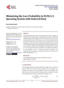
Figure 1: A layered queueing network model of web server connected to two lower-level servers.

• The Clients, which have the role of customers, are a set of Tasks running on desktop computers. Customers in the model are assumed to cycle forever. The Clients are indicated as a set of tasks by showing a “stack” of task images, with the parameter “{y}” to indicate y Clients. • The processor which serves to execute each task is indicated by a “host” association, shown by an arrow labelled “(h)”. The processor demand for each entry is defined as a pair “[s1, s2]” giving the average amount of CPU demand for phase one and phase two. The average processor demand has an exponential distribution by default, but a coefficient of variation can be specified. • The mean number of requests from one task to a lower layer task are indicated on the request arc by a pair “(y1, y2)” for requests phase one and phase two. The number of requests can either be geometrically distributed, with the given mean, or can be an exact number. Other features of the model, such as heterogeneous threads and asynchronous messaging, are not described here.

Analytic Solution to choose which approximations to use. This may involve a tradeoff of accuracy and computational effort. After describing layered modeling and the value of a second phase of service, this paper assembles three approximations for delay at a multiserver with a second phase of service and compares them for accuracy and solution time. One approximation is found to be the best compromise of accuracy and speed. Using this approximation, a substantial model study of the Network File System (NFS) is described, to show how multithreading and deferred service improves its performance.

Layered Queueing Networks A layered queueing network is a kind of Extended Queueing Network with a layered structure. A server A, in the midst of serving a customer, can make requests for service from a server B at a lower layer. During the service by B, the customer and server A are both inactive. We can regard this as a state in which the customer holds both servers, so the essence of layered queueing is a form of simultaneous resource possession. Layering arises if there is a partial order among the servers, such that service by “lower” servers is nested within service by “upper” servers. Fig. 1 illustrates several of the features of a Layered Queueing Network model using a simplified model of a web server. • The model is defined by a set of entities called “tasks” which act as customers and servers, linked by arrows indicating requests or associations. Hardware servers (processors) are shown in the Figure as circles, the rest are parallelograms. • The small parallelograms within tasks are called “entries” and are used to differentiate services provided by tasks. The solid arrow with a filled head between entries indicates that the sender blocks (waits for a reply), for example, the web client waiting for the requested page to be delivered.

A layered queueing network is solved analytically by splitting the original model into set of closed queueing network “layer submodels”, with implicit relationships between their parameters (as used in Extended Queueing Networks using surrogate delays). Each layer submodel contains as servers, the servers at a given call depth or request depth from the clients [20, 6, 12]. As customers, it contains surrogates for all the customers of these servers. A single-threaded higherlevel task gives rise to a customer chain with one customer; a multi-threaded task gives a chain with a customer for each thread. Submodels are solved using an approximate MVA algorithm such as linearizer [3]. The parameters of a layer submodel are found partly from other layers: • The service times of its servers are calculated from waiting times and service times in lower layers. • The time between requests from the customers of a chain is a surrogate delay or “think time” for the chain, which is determined by the frequency of requests and other behaviour of the corresponding upper layer entity. The web of relationships by which results are found in one layer and used in another layer is resolved by a fixedpoint iterative calculation, which has been described in other papers [20, 6, 12]. The overall strategy has been applied to many models and generally converges well (sometimes under-relaxation must be used), with approximation errors of a few percent.

Performance Impact of Second Phases The difference between ordinary one-phase service, and twophase service (which was originally introduced in layered models in [19]), is explained in Fig. 2. The server replies to its clients as early as possible, then continues to execute the remainder of the request in parallel with the client. The model in Fig. 1 will be used to show how second phases can

Client Server

Send Receive

Send Reply

Receive

Ph 1

Ph 1

(a) Single Phase Service Client Server

Send Receive Ph 1

Send Reply

deemed the most suitable and are modified here to account for the second phase of service. The delay, W , for a customer in chain k at a two-phase, multiclass multiserver j at a customer population N has the following components [5]: 1. its own service time, Skj ,

Receive

Ph 2

Ph 1

(b) Two Phase Service

Figure 2: Standard Remote Procedure Call with One and Two Phases of Service

2. the time spent waiting in the queue (effective backlog), xe, and 3. the time spent waiting for a server to become free (departure time), xr. and is calculated using:

improve response times. The number of Clients, y, and the fraction of phase-2 service time, x, are both varied. All other parameters are set to the values shown in the figure. The response time and utilization of the web-server are shown in Fig. 3. Results were generated using both simulation, and the analytic approximations described below. These results show that the second phase may have a large or a small effect. When the number of available threads exceeds the number of potential customers, two-phase multiservers can offer substantial performance benefits. However, when heavy queueing occurs at the two-phase multiserver, as in Fig. 3(d), second phase service offers little or no performance improvement.

Two-phase Multiclass Multiservers This section describes the impact of second-phase service on the calculations for multiclass multiservers which were explored for simple load-independent servers in [20, 12]. These servers need new waiting time expressions to compensate for two factors. First, the client is not held for the entire period of execution of its request at the server, shown in Fig. 2(b). Second, a client making a subsequent request to a server may block while the server completes its own preceding request. This phenomenon is called overtaking and is shown in Fig. 4. Submodels that arise from layered queueing networks often have sets of clients that make different demands on the servers. Further, software servers usually have first-come, first-served (FCFS) queueing disciplines. The corresponding queueing network model must therefore have FCFS service centers with service demands that vary by chain. Queueing networks with these characteristics do not have a product form solution. Fortunately, approximations exist for multiclass FCFS single- and multiple-servers which are sufficiently accurate for practical purposes [11, 13, 5, 1, 14, 12]. The waiting time expressions described in [13, 5, 12] were Client Server

Send Receive Ph 1

Send Reply

queue

Ph 2

Service

Receive Ph 1

Figure 4: Overtaking occurs when a client is queued because a server is still processing the client’s previous request.

Wkj (N)

=

Skj +

K X

xekcj (N)Qcj (N − ek )

c=1

+ PBj (N − ek )xrkj (N)

(1)

This expression will be modified for two phases of service first since it is the most detailed of [13, 5, 12] . The first term is changed to Skj1 , the phase one service time, since the customer is not delayed by its own second phase of service at the server. The second term is the delay which arriving customers see, prior to being serviced caused by other customers waiting in the queue Qcj (N − ek ). With a multiphase server, servers busy in phase two, Ukj2 are equivalent to “new” customers that are created when replies to clients are sent. New arrivals must also wait behind these pseudo customers. The third term, the departure time, includes both phases of service, so it is unchanged, and depends on the probability that all servers are busy, PBj (N − ek ). The second effect that must be taken into consideration is overtaking. The probability of overtaking, Pr{OT }kj , is the probability that a customer from chain k finds server j busy processing phase two of an earlier request from that same customer. This probability is calculated based on the race between • γkj , the time from the customer’s departure from server j and its next return, and • Skj2 , the duration of phase two of the server. If these times are assumed to be exponentially distributed, this probability is [20, 12] Pr{OT }kj =

1/γkj 1/γkj + 1/Skj2

(2)

Equation (2) calculates the probability that some server is still doing a previous phase two for this customer, when it returns. The total work having to be done before the job enters is then increased by one second phase, and this is spread across the Mj servers, the same as the work in the queue is spread in some of the approximations. This probability is multiplied by the phase two service time, Skj2 , to find the overtaking delay.

0.8

0.6 0.6

0.5 0.4

0.4

0.3 0.2

1.2

5 4

1 0.8

3

0.6

2

0.4

0.2

1

0.2

0.1 0

0 0.2

0.4 0.6 0.8 Fraction Phase 2 Service

0

1

0 0

0.2

(a) 10 Clients 7.7

30

1.5

20

1

Response Time

40

2

50

Sim R LQN R Sim U LQN U

7.65 Server Utilization

2.5

1

70 Clients, 50 Servers 50

Sim R LQN R Sim U LQN U

3

0.8

(b) 30 Clients

50 Clients, 50 Servers 3.5

0.4 0.6 Fraction Phase 2 Service

7.6

40

7.55

30

7.5

20

7.45

10

Server Utilization

0

Response Time

6

Sim R LQN R Sim U LQN U

1.4 Response Time

0.7

1.6

Server Utilization

0.8

Response Time

30 Clients, 50 Servers 1

Sim R LQN R Sim U LQN U

Server Utilization

10 Clients, 50 Servers 0.9

10

0.5

7.4

0

7.35 0

0.2

0.4 0.6 0.8 Fraction Phase 2 Service

1

0

0.2

(c) 50 Clients

0.4 0.6 0.8 Fraction Phase 2 Service

1

(d) 70 Clients

Figure 3: Client response time and Web Server utilization versus fraction of phase two service time for the model in Fig. 1. Simulations were conducted with 95% confidence intervals of ±1%. The analytic solutions were performed using (3).

to handle multiple classes and second phases:

After these changes, Equation (1) becomes: Wkj (N)

= +

(1)

Skj1 K X

Wkj (N)

xekcj (N)[Qcj (N − ek ) + Ucj2 (N − ek )] ×

c=1

+ +

PBj (N − ek )xrkj (N) Pr{OT}kj · Skj2 Mj

= +

(3)

" K X 1 Scj [Lcj (N − ek ) Skj1 + Mj c=1

Ucj2 (N − ek )] Mj −2

+

Sj

X

(Mj − 1 − i)Pj (i, N − ek )

i=0

+

Pr{OT}kj · Skj2 Mj



Skj1 + K X

Uj (N − ek )M Mj

Scj [Lcj (N − ek ) + Ucj2 (N − ek )]

c=1

Reiser’s multiserver expression [11], modified by [13] for multiple classes, is modified further for second phases in a similar fashion:

Wkj (N)

=

(4)

Rolia’s multiserver expression [12], is modified here both

+

Pr{OT}kj · Skj2 Mj

(5)

Accuracy and Performance Comparisons This section explores the accuracy and performance of the two-phase multiclass multiserver approximations using two models. The first model, shown in Fig. 5, is a simple singleclass system used to study accuracy based on the utilization and fraction of phase two service at the server. The number of clients, x, was varied from 1 to 10, the number of servers, y, was varied from 1 to 5, and the and the fraction of phase one service time, p, was varied from 0 to 1. Fig. 6 shows contour plots of the error in throughput (ǫλ = apprx−sim × 100) for the three approximations desim scribed above. Equations (3) and (5) are clearly superior to (4). The algorithms are least accurate when the server is fully saturated and has a high percentage of phase two service. The second model was adapted from [4] to evaluate the behaviour of the new approximations using multiple chains and multiple classes of service (the original queueing network was used to evaluate (1)). Service times for each phase

ǫλ (%)

0.00 0.07 0.07 0.03 0.14 0.18 0.03 0.17 0.20 0.02 0.48 0.36 0.03 0.53 0.54

ARE (%) 1.34 5.09 4.92 1.59 4.08 4.41 1.62 4.99 4.67 1.66 6.30 5.33 1.77 7.24 5.88

Run Time 42:44.5 7:05.1 15.0 5.9 3:43.0 5.6 8.8 3:43.5 5.1 6.1 3:47.3 5.4 6.2 4:22.0 12.0 4.4

1 0.8 0.6 0.4 0.2 0

0.2 0.4 0.6 0.8 Fraction Phase 1 Service Time

1

(a) Equation (3) 1 0.8 0.6 0.4 0.2 0

0.2 0.4 0.6 0.8 Fraction Phase 1 Service Time

1

0

1 0.8 0.4

0

This section describes a Layered Queueing Network model of the Network File System [2] (V2) implementation in the Linux kernels. First the LQN model is described and validated. Next, some performance predictions are made using the model (and tested against the live system where possible).

c1 [0,2] c1 {x} (0,1)

e1 [p1,(1−p1)] s1 {y}

Figure 5: Single Class test case.

0.2 0.4 0.6 0.8 Fraction Phase 1 Service Time

1

Utilization

0.6 0.2

Layered Queueing Model of NFS

10 5 −5 −10 −25

(b) Equation (4)

Table 1: Performance Results for two phase multiclass multiservers. Simulations were conducted with 95% confidence intervals of ± 1%.

of service at each of the lower-level servers were chosen randomly from a range of values between 1.275 and 36.195. Two hundred different networks were tested with the fraction of phase two varying from 0.04 to 0.96. Another two hundred test cases were run with phase two fractions fixed at 0.25, 0.50, 0.75 and 1.00 for fifty cases each. The number of visits to each of the servers was varied from 0.35 to 2.30. Table 1 shows the results from using the second model. ǫλ is as above, ARE is the Absolute Relative Error in throughput × 100) and the Run Time is the average (ARE = |apprx−sim| sim time to run a test case. Based on the ARE metric, (3) is more accurate than either (4) or (5), but much more computationally expensive.

25 10 5 −5

0

Utilization

-0.66 0.10 0.96 -0.80 -0.59 0.60 -0.83 0.93 0.64 -0.84 1.87 1.12 -0.79 3.62 0.94

σ

Utilization

Eqn %Ph2 Simulation (3) rand (4) (5) (3) 25 (4) (5) (3) 50 (4) (5) (3) 75 (4) (5) (3) 100 (4) (5)

10 5 −5

0

(c) Equation (5)

Figure 6: Single class test case throughput error contour plots.

Performance Model The workload for the model was based on the the mix of operations used by nfsstones benchmark [15] though the file sizes were increased by an order of magnitude to account for the increased memory sizes in today’s machines. The read, write, and lookup functions dominate the workload, so only these operations were modeled. UML sequence diagrams of these operations are shown in Fig. 7. Note that lookup and read use synchronous operations (Fig. 7(a) and (b)) while write uses asynchronous messages (Fig. 7(c)). The asynchronous behaviour permits the client to proceed once the data is written to the local system’s buffer cache and improves performance substantially, but does not adhere to the NFS specification. The layered queuing network model for Linux NFS is shown in Fig. 8. It is divided up into four principle components: the client, the network, the file server and the disk. nfsstone, nfsiod and rpcnfsiod are all actual Linux processes. Clientcache and servercache represent the buffer pool and have two phases of service representing read-ahead and writebehind for reads and writes respectively. Parameters were found through instrumentation of the Linux V2.0 kernel while running nfsstones, though runs with the V2.6 kernel show no substantial change in performance. The network task represents the delay caused by the Ethernet. The model here is from [9] modified to account for the fact that an Ethernet with large packets is about 83% efficient [17]. The disk task represents the actual disks. Two buckets were used: one grouping

:Client

:rpc.nfsd

:Disk

main [95.7]

lookup opt

[cached=no] read

nfsstone{60} (0.63)

(a) Lookup :Client

:nfsiod

c_read [50.9]

:rpc.nfsd

:Disk

[cached=no] read opt

c_write [76.1,2]

clientcache{400}

read opt

(0.06)

(0.11) [cached=no] read

b_read [11.8] (0.496) nfsiod{4} (0.63) (0,7)

(b) Read :Client

:rpc.nfsd write

(4)

:Disk

(0.124)

(1) (0.31)

n_read [410.4]

ether [208.3]

lookup [415.9]

client

rpcnfsd (1)

(c) Write

Figure 7: Sequence Diagrams of major NFS operations. nfsiod and client execute on the client’s processor. rpc.nfsd executes on the file server. (a) Throughput

Live LQNS Sim.

n_write [410.4]

write

network

Method

(0,1)

NFSstones λ ǫλ (%) 2820 N/A 2984 5.82 2883 2.23

Solution Run Time 11:15.00 11.98 2:02:56.80

(0.5)

s_read [20.8,2]

(1)

s_write [39.1,2]

servercache{400} (0,0.0061) (0.00084,0.0222) (0,0.0558) (0.00133,0.035) d_read [6910]

d_read_4k [10560]

d_write [11780]

d_write_4k [2440]

server

disk

Figure 8: Layered Queueing Network of principle NFS operations.

(b) Utilization

Component client server disk network

Utilization Live LQNS 0.36 0.40 0.59 0.67 0.53 1.00

Table 2: Base model results. The simulations were run with a 95% confidence interval of ± 5.0% for each of the entry’s service times.

reads and writes of 4KBytes, and a second for everything else. The model in Fig. 8 was solved analytically (shown below as LQNS) and by simulation to find the throughput at the client. The results are compared to the average of twenty live runs performed on a private switched network in Table 1(a) for both accuracy and run time (the run time given for the live run is the sum of the twenty runs). Table 1(b) shows the utilization of all of the four principle components in Fig. 8. The performance model clearly shows that the Ethernet is the bottleneck in the system.

Performance Predictions The base model described above was varied in a number of ways to study the effect of possible changes in the system. The changes were analyzed using the workload described earlier (“Base”), the Laddis workload [18] (“Laddis”), and with the Laddis workload using a network which is ten times faster than the 100Mb one analyzed here (“Fast”). Synchronous Writes The NFS protocol specification states that writes are to be committed to stable storage before the server replies to the client. The Linux NFS implementation simply waits for the write request to complete to the local buffer cache then replies; the disk block is actually written a short time afterwards. To properly implement NFS, rpc.nfsd was modified to perform synchronous writes on the live system. The LQN model was modified as follows. 1. All writes from the server’s buffer cache were moved to phase one from phase two. 2. Each write is assumed to take the same time as a 4K Read. The extra time allows for seeking and rotational delays. 3. Each 8K write results in two write requests: one for the

Client Model Base

Laddis Fast

Method Live LQNS Sim. LQNS Sim. LQNS Sim.

NFSstones (λ) Base Synch. 2820 1072 2984 538 2883 848 1947 254 1906 406 2566 254 2653 406

Change (%) −61.99 −81.97 −70.59 −86.95 −78.67 −90.10 −84.66

Client Model Base Laddis Fast

Method LQNS Sim. LQNS Sim. LQNS Sim.

NFSstones (λ) Base 8K Read 2990 3173 2884 3054 1947 1973 1906 1930 2565 2654 2653 2733

Change (%) 6.10 5.89 1.34 1.25 3.43 3.01

Table 5: Comparison of 8K Read Requests to Base model. Table 3: Comparison of Synchronous Writes to Base model. Client Model Base Laddis Fast

Method LQNS Sim. LQNS Sim. LQNS Sim.

NFSstones (λ) Base Gather 2990 2977 2884 2787 1947 1940 1906 1895 2566 2214 2653 2213

Change (%) −0.44 −3.35 −0.36 −0.57 −13.72 −16.55

Table 4: Comparison of Synchronous Writes with Gathering to Base model.

meta data in the inode, and one for the actual data. Both writes must complete synchronously. The results, shown Table 3, show a significant degradation in performance. Even though writes make a small fraction of the workload, their behaviour has a significant effect on the performance of NFS. Synchronous Write Gathering Write gathering [8] is a technique used to improve NFS performance while retaining the synchronous write semantics. Writes to the disk, and replies to the client, are delayed by rpc.nfsd in the hope that additional write requests will arrive a short time later. The goal is to merge the requests into one large operation thus saving significant amounts of disk activity from meta data updates intermixed with data updates. To model synchronous writes, the base model was modified by moving the write requests at the server’s buffer cache from phase two to phase one. The write performance from the base model is retained. The results, shown in Table 4, show that write gathering has significant performance benefits. However, when the network performance is improved to the point where it is no longer the bottleneck, synchronous writes still impact performance. Big Reads The Linux 2.0 NFS implementation performs reads in chunks no larger than 4K bytes, even if the rsize mount parameter is larger than this value. This behaviour is an artifact of the file system implementation because the virtual file system makes read requests on a 4K page basis. Conversely, the largest write request is limited only by the wsize mount parameter. Larger requests can improve performance by reducing network traffic.

To study the performance impact of RPC read requests which are twice as large, the model was modified as follows: 1. The call rates from the client’s buffer cache read to nfsiod and rpc.nfsd were halved to reflect the larger reads. The number of requests to the Ethernet was changed to reflect the larger read size. 2. The call rates from the client buffer cache’s read to ether was changed from four packets per request to seven packets per request. 3. The request rates from the server’s buffer cache read to the disk were doubled because each read request is now twice as large. Table 5 shows the estimated performance improvement from this change. The base model shows the biggest performance improvement because the Ethernet is the bottleneck and the workload is skewed towards reads. When the Laddis workload mix is used with the 100Mb Ethernet, there is very little difference between the base and 8k-read throughput results because this workload has less read activity. However, with a faster Ethernet, the larger read request size shows more improvements.

Conclusions This paper has introduced the analysis of two phase multiservers with one or more classes. Two-phase servers, which reply to a client prior to completing all of the work requested by that client, can be useful for improving the performance of a system, provided that the server is not saturated. Three multiclass multiserver waiting time expressions (i.e., those which allowed for chain-dependent service times and FCFS scheduling) were modified to allow for two-phase server operations. All three approximations had good accuracy when compared to simulation, with approximation errors of less than 7% on average. When run-time efficiency is considered, (5) is the best choice. This expression scales exceptionally well because it does not rely on the marginal probabilities. The results presented here were studied in Layered Queueing Networks because this type of queueing network is a convenient way of analyzing the performance of a multi-tier client-server system. However, Layered Queueing Networks are solved using conventional queueing networks, so the new residence time expressions can also be used to solve a conventional queueing network.

Acknowledgments This research was supported by the Natural Sciences and Engineering Research Council of Canada and by Communications and Information Technology Ontario (CITO).

References [1] S. C. Bruell, G. Balbo, and P. V. Afshari. Mean value analysis of mixed, multiple class BCMP networks with load dependent service centers. Performance Evaluation, 4:241–260, 1984. doi:10.1016/0166-5316(84)90010-5. [2] B. Callaghan. NFS Illustrated. Addison Wesley, 2000. [3] K. M. Chandy and D. Neuse. Linearizer: A heuristic algorithm for queueing network models of computing systems. 25(2):126–134, Feb. 1982. doi:10.1145/358396.358403. [4] A. E. Conway and D. O’Brien. Validataion of an approximation technique for queueing network models with chain-dependent FCFS queues. Computer Systems Science & Engineering, 6(2):117–121, Apr. 1991. [5] E. de Souza e Silva and R. R. Muntz. Approximate solutions for a class of non-product form queueing network models. Performance Evaluation, 7(3):221–242, 1987. doi:10.1016/0166-5316(87)90042-3. [6] G. Franks, A. Hubbard, S. Majumdar, D. Petriu, J. Rolia, and M. Woodside. A toolset for performance engineering and software design of client-server systems. Performance Evaluation, 24(1–2):117–135, Nov. 1995. doi:10.1016/0166-5316(95)96869-T. [7] G. Franks and M. Woodside. Effectiveness of early replies in client-server systems. Performance Evaluation, 36(1):165–184, Aug. 1999. doi:10.1016/S0166-5316(99)00034-6. [8] C. Juszczak. Improving the write performance of an NFS server. In Proceedings of the Winter 1994 USENIX Conference, pages 247–259, San Francisco, CA, Jan. 1994. USENIX Association. [9] E. D. Lazowska, J. Zhorjan, S. G. Graham, and K. C. Sevcik. Quantitative System Performance; Computer System Analysis Using Queueing Network Models. Prentice Hall, Englewood Cliffs, NJ, 1984. [10] J. E. Neilson, C. M. Woodside, D. C. Petriu, and S. Majumdar. Software bottlenecking in clientserver systems and rendezvous networks. IEEE Trans. Softw. Eng., 21(9):776–782, Sept. 1995. doi:10.1109/32.464543. [11] M. Reiser and S. S. Lavenberg. Mean value analysis of closed multichain queueing networks. J. ACM, 27(2):313–322, Apr. 1980. doi:10.1145/322186.322195. [12] J. A. Rolia and K. A. Sevcik. The method of layers. IEEE Trans. Softw. Eng., 21(8):689–700, Aug. 1995. doi:10.1109/32.403785.

[13] A. R¨uth. Entwicklung, Implementierung und Validierung neuer Approximationsverfahren f¨ur die Mittelwertanalyse (MWA) zur Leistungsberechnung von Rechnersystemen. Diplomarbeit am IMMD der Friedrich-Alexander-Universit¨at Erlangen-N¨urnberg, 1987. [14] R. Schmidt. An approximate MVA algorithm for exponential, class-dependent multiple servers. Performance Evaluation, 29, 1997. doi:10.1016/S0166-5316(96)00048-X. [15] B. Shein, M. Callahan, and P. Woodbury. NFSSTONE: A network file server performance benchmark. In USENIX Summer 1989 Technical Conference Proceedings, pages 269–275, Baltimore, MD, June 1989. USENIX Association. [16] C. E. Skinner. A priority queueing system with serverwalking time. Operations Research, 15(2):278–285, 1967. doi:10.1287/opre.15.2.278. [17] J. Wang and S. Keshav. Efficient and accurate ethernet simulation. Technical Report TR99-1749, Computer Network Research Group, Cornell University, Ithaca, NY, May 1999. [18] M. Wittle and B. E. Keith. LADDIS: The next generation in NFS file server benchmarking. In USENIX Summer 1993 Technical Conference Proceedings, pages 111–128, Cincinnati, OH, June 1993. USENIX Association. [19] C. M. Woodside. An active-server model for the performance of parallel programs written using rendezvous. In Proc. IFIP Workshop on Performance Evaluation of Parallel Systems, Grenoble, Dec. 13–15 1984. [20] C. M. Woodside, J. E. Neilson, D. C. Petriu, and S. Majumdar. The stochastic rendezvous network model for performance of synchronous client-server-like distributed software. IEEE Trans. Comput., 44(8):20–34, Aug. 1995. doi:10.1109/12.368012.