Design and Implementation of a Fuzzy-Based Gain ...

2013 12th Mexican International Conference on Artificial Intelligence

Design and Implementation of a Fuzzy-Based Gain Scheduling Obstacle Avoidance Algorithm Luis C. Gonzalez-Sua, Olivia Barron, Rogelio Soto, Leonardo Garrido, Ivan Gonzalez, J. L. Gordillo and Alejandro Garza Tecnol´ogico de Monterrey Monterrey, NL, Mexico 64849 Email: [email protected], [email protected], [email protected], [email protected], [email protected], [email protected], [email protected] Abstract—This article presents a novel obstacle avoidance algorithm. Using a combination of fuzzy logic and gain scheduling theories, a new methodology that reduces computational costs compared to conventional fuzzy methodologies, specially when the variables to be controlled are too many. For comparison purposes, a potential field algorithm was implemented. Both algorithms are tested in a series of experiments to determine if the new algorithm is at least as good as the potential field algorithm. The metrics defined for these experiments are: the number of times that the agent collides (collisions), the time spent to finish a traced course (time spent) and the remaining stamina of an agent at the end of an experiment (stamina consumption). The results show that the proposed algorithm achieve a low level of collisions. Also, the proposed algorithm shows a considerable improvement in the time spent for the completion of the proposed tasks. Last but not least, the results demonstrate a considerable reduction in the stamina consumption using the proposed algorithm over the potential field algorithm.

I.

needs to correct its course. In some cases, due to unforeseen situations, the agent/robot is too close to the obstacle, and a drastic evasion is needed. Among the most common evasive maneuvers currently used are the following: strafing to a side (this only applies to some legged and steered mobile robots) and coming to a total halt and suddenly change direction (it applies for differential robots). In this article an algorithm is proposed. This algorithm not only can make course corrections and can also take evasive maneuvers if the situation needs it. The article is divided in four more sections: related work, proposed methodology, experiments and results and at the end, conclusions and future work. II.

Among the most common used algorithm there is the potential fields algorithm, which uses the rejection/attraction theory of the magnetic fields to maintain distance between the agent and any obstacle, and attract the agent to the goal. There are several obstacle avoidance algorithms currently developed [7], but for comparison purposes this section will focus on potential fields algorithm (PFA) and the theory of the proposed algorithm in this article, the fuzzy logic algorithms (FLA).

I NTRODUCTION

Obstacle Avoidance is an attention demanding task, mainly because it involves several other minor tasks. Among them, there is awareness of the surroundings, course correction and in some cases, evasive maneuvers (it applies when the space is too tight for the course correction to elude collision). The order of execution of the formerly mentioned tasks is the following. First of all it is necessary to spot the obstacle, there is no chance to avoid something if there is no knowledge of the whereabouts of it [4]. After the obstacle has been detected, a subtask is implemented to predict the movement of the obstacle, in other words to calculate its possible trajectory. If the obstacle is static then the trajectory will be null. However, if the obstacle is moving, calculating speed and direction is crucial to determine the obstacle’s next location; though sometimes, getting that information is not possible either because the obstacle’s movement is erratic or because it is too far to get an accurate measurement.

A. Potential Fields algorithm As mentioned before, PFA uses the magnetic fields theory. For obstacles and objects to be avoided, a rejection potential is used. For goal or other desired locations or objects, an attraction potential is employed. Equation (1) shows how the −−→ → q1 is potential rejection/attraction value Upot is calculated. − → the rejection/attraction values for obstacle/target and − q2 is the rejection/attraction value for the agent and d is the distance between the obstacle/target and the agent. Notice that all of the values except the distance are vectorial, so the resultant potential field will be a vectorial value indicating where the potential field is moving the agent.

Once trajectory has been predicted, or at least the possible whereabouts in the future, the course correction kicks in and alters the course just enough to avoid collisions, but not too much to get too far from the initial goal path [6]. To decide how much course correction is needed, there is a decision making process that must take into account the information received in the previous task and then decide how much the agent/robot 978-1-4799-2605-3/13 $31.00 © 2013 IEEE 978-1-4799-2604-6/13 DOI 10.1109/MICAI.2013.11

R ELATED W ORK

→ − q2 q1 × − −−→ → Upot = 2 d

(1)

Due to the simplicity and low processing costs of the potential fields algorithm, it is often the most common choice 45

Fig. 1. Block Diagram of the Fuzzy-Based Gain Scheduling algorithm, notice how the output of the previous stages goes to the next stage.

(a) Effort’s MFs

[9]. However, that algorithm has a considerable disadvantage, it is vulnerable to local minima. Using different heuristic techniques like simulated annealing or harmonic functions, that vulnerability to local minima can be reduced[7]. B. Fuzzy Logic Algorithm Fuzzy logic emulates human thinking using fuzzy values instead of crisp values, for example, instead of saying that speed is 10 km/h, fuzzy logic determines speed as slow. To convert a crisp value like 10 km/h to a fuzzy value, a previously defined membership function define the membership degree in a range from 0 to 1 for each crisp input value. Once the input values are fuzzified, the fuzzy inference engine comes into action. For each input function, there is a corresponding rule. The membership value determines which rules are activated and the output value is calculated according to the output membership function of each activated rule. The process of converting fuzzy values to a crisp value is known as defuzzification.

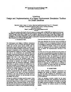
(b) Stamina’s MFs Fig. 2. Membership functions for inputs of Stage 1. Figure 2(a) is the effort’s MFs, solid line is for Tired and Dashed line is for Fresh. Figure 2(b) is the stamina’s MFs, solid line is Critical, dashed line is Normal and doted line is High. TABLE I.

Currently, fuzzy logic is used for some obstacle avoidance applications [1], [6], also, due to the fuzzyfication and defuzzyfication processes, a noise reduction is obtained. Because of that, no filtering stage is required, and chattering in the output is considerably reduced [10]. III.

Stamina Critical Normal High

RULES FOR S TAGE 1 Effort Tired Fresh Slow Sprint Slow Sprint Jog Sprint

The second stage controls if the agent stays in course or makes any correction, either changing direction or making a strafe (move to the side without changing the body direction). This stage helps to reduce overcorrection, therefore, improving the time spent to reach the target. The inputs of the second stage are the Distance (distance to the obstacle) and the Relative Speed (the speed with which the agent approaches the obstacle). Figure 3 shows the MFs for the Distance and Relative Speed inputs. Table II shows the rules for Stage 2. Outputs for stage 2 determines the agent evasive action. If the output is Stay, the agent must do nothing, in order to avoid overcorrection. Turn determines that the agent must do course corrections and Strafe the agent must move to a side without changing the body direction.

P ROPOSED M ETHODOLOGY

The proposed methodology is for a fuzzy-based algorithm with gain scheduling. The gain scheduling is implemented to reduce the number of evaluated rules without the sacrifice of the model’s structure. The controller is divided in three stages, as shown on figure 1. The first stage receives as input the effort and the stamina values. The effort is a value the simulator uses to emulate the effect of fatigue in the agent. If effort is at maximum, the agent can reach maximum velocity, but if it is less than maximum, the agent can only reach the proportional amount of speed, but at the same cost of energy as it was at full effort. The range of the effort is from 0 to 1. The stamina is the energy of the agent. The agent consumes stamina proportionally to the power of the dash, each time it accelerates, . The range of the stamina is from 0 to 8000. Figure 2 shows the membership functions (MFs) for the inputs of stage 1. Table I shows the rules for the Stage 1. The output values determines the acceleration output, Sprint is for maximum acceleration, Jog is for medium acceleration and Slow is for minimum acceleration.

TABLE II. Rel. Speed Away Slow Fast

RULES FOR S TAGE 2 Distance Very Close Close Strafe Turn Strafe Turn Stay Stay

Far Stay Stay Stay

The third and final stage is in charge of selecting where the

46

(a) Distance’s MFs

(a) Direction’s MFs

(b) Relative Speed’s MFs

(b) Angular Speed’s MFs

Fig. 3. Membership functions for inputs of Stage 2. Figure 3(a) is the distance’s MFs, solid line is for Very Close, Dashed line is for Close and doted line is for Far. Figure 3(b) is the Relative Speed’s MFs, solid line is Away, dashed line is Slow and doted line is Fast.

Fig. 4. Membership functions for inputs of Stage 3. Figure 4(a) is the Direction MF’s, solid line is for Far Left, dashed line is for Left, doted line is for Center, dashed-doted line is for Right and diamond Line is for Far Right. Figure 4(b) is the Angular Speed MF’s, Solid Line is To Left, dashed line is Static and doted line is To Right.

correction will be applied, (i.e. go left, go right or straight), and according to the stage 2, the action will be a strafe/turn to the left/right or no strafe/turn at all. This stage has as inputs the current position of the obstacle and the relative Angular Speed (this speed is not measured in degrees/sec or radian/sec, is more like an orthogonal speed). Figure 4 shows the MF’s of the Stage 3. Table III shows the rules for the Stage 3. The Go Side option is a wild card option, it varies according to the location of the agent. If the agent is closer to the left side, it will select Go Right and vice versa, however, for general purposes, it can be replaced by either Go Right, or Go Left or a random option between those two. The reason why it is a wild card, is because both options are equally good, and there is no other input that can make one option better than the other one. TABLE III. Direction Far Left Left Center Right Far Right

IV.

To measure the effectiveness of the algorithm, three metrics were proposed: Time Spent(game cycles), Stamina Consumption (agent’s stamina) and collisions (number of times that the agent touches an obstacle). To test these metrics, three experiments were designed, each one focused in measuring a particular value, although, all of the metrics were also measured in all of the experiments. All of the experiments were implemented in the Robocup Simulation 2D environment [5]. The time spent metric is the number of the cycle when the experiment ends minus the cycle number when the experiment starts. The stamina consumption was determined by the difference of the stamina pool of the agent at the beginning of the experiment minus the stamina pool at the end of it. The stamina pool is a variable of the agent, that determines the total value of stamina, it only decreases; the agent has a stamina value but it can increase or decrease according to the actions it develops, and the stamina available in the stamina pool. Collisions are counted every time the simulation environment considers a collision, that occurs when the agent try to occupy the same space as an obstacle. For the collision’s metric they are not only counted any time it occurs, they are also added as penalties of ten cycles of time in the time spent metric.

RULES FOR S TAGE 3

To Left Straight Straight Straight Go Right Straight

Angular Speed Static Straight Straight Go Side* Straight Straight

E XPERIMENTS AND R ESULTS

To Right Straight Go Left Straight Straight Straight

The values of the MF’s were obtained analytically, and rules were selected by common sense, however, because of the noise, further tuning of the MF’s is required to improve performance.

For comparison purposes, the comparing algorithm is potential fields. It was selected because is one broadly used

47

Fig. 6. Layout for experiment 2, the circuit has three obstacles, two dynamic and one static at the center. R ESULTS E XPERIMENT 2

TABLE V. Simulations

100

Fuzzy Logic Potential Fields

Fig. 5. Layout for experiment 1, the circuit has six obstacles, three static at the top and three dynamic at the bottom.

The third and last experiment was designed to test the algorithm in an aggressive approach. The obstacle will find the agent and try to tackle it. Figure 7 shows the layout of the experiment. This experiment is quite simple, the aggressive obstacle waits the agent in the middle of the field and then goes and tries to tackle the agent unless the agent reaches a safe limit. Table VI shows the results of the experiment.

The first experiment takes more game cycles than the other experiments. It was designed to test the stamina consumption, that is why it is longer. In this experiment, the agent must go through a defined course with six obstacles, three static obstacles and three moving obstacles. Figure 5 shows the experiment layout with the obstacles’ coordinates.

Fuzzy Logic Potential Fields

TABLE VI. Simulations

R ESULTS E XPERIMENT 1 100

Time Spent Avg. 341.92 527.9

Stamina Avg. 14705.85 17388.33

Collisions Avg. 0.47 0

C. Experiment 3

A. Experiment 1

Simulations

Stamina Avg. 4580 8779.45

consumption, almost at half, however, the collision reduction is not as good as the potential field’s one.

algorithm, it is simple to implement and effective, has a very low computational processing cost and is considered among the best current obstacle avoidance algorithms [9].

TABLE IV.

Time Spent Avg. 109.57 187.02

Fuzzy Logic Potential Fields

Collisions Avg. 1.46 0.1

R ESULTS E XPERIMENT 3 125

Time Spent Avg. 114.35 151.93

Stamina Avg. 4408.56 6173.60

Collisions Avg. 0.41 0.28

Results show that for both algorithms, avoiding the incoming obstacle is not a simple task, both agents were hit. For the potential fields, the collision average is less, but it consumes a 50% more stamina than the Fuzzy algorithm, and the time spent is also almost a 50% more. The higher collision value of the fuzzy algorithms is an indisputable evidence of the need of further tuning.

Results in table IV show that the potential field algorithm successfully avoids obstacles, however, sometimes makes a kind of a cheat, because it doesn’t go through the moving obstacles, instead it goes around them. It is effective to reduce collisions, but at a great cost in time and stamina. On the other hand, the fuzzy algorithm dramatically reduces the stamina consumption and the time spent, however, the average collisions are not as good as expected, suggesting that a more meticulous tuning is required.

V.

C ONCLUSIONS AND F UTURE W ORK

Despite that the results weren’t as encouraging as expected, the algorithm shows a better management of stamina and time spent to complete the task. As mentioned several times before, the results undoubtedly show that the fuzzy algorithm needs more meticulous tuning, however, the tuning process can be repetitive and strenuous, for a user. Nevertheless, applying Genetic Algorithms or Q-Learning, can do such task quite easily and obtain better results than the human user.

B. Experiment 2 The second experiment is shorter than the first one, it was designed to measure the time that the agent spends to finish an assigned course. The course for this experiment is a straight line with three obstacles, two of them are dynamic, located at the beginning and at the end of the line, and one static obstacle located in the middle. Figure 6 shows the experiment 2 layout. Table V shows the results for this experiment. Results show that again the potential field does the cheating of not going in a straight line through the obstacles, and again at a great cost in stamina consumption and time, however, it is effective to avoid collisions. On the other hand, the fuzzy algorithm reduces considerably the time spent and the stamina

Fig. 7. Layout for experiment 3, the circuit has only one aggressive obstacle that will attempt to collide with the agent.

48

Once a well tuned and functioning algorithm is obtained, it can be implemented in mobile robots, like E-puck’s, Turtlebot’s or NAO’s, but, the data acquisition must be improved. Noise cannot only reduce the effectiveness reducing collisions, but can also make the algorithm less effective in stamina (power) consumption or time spent to finish the task. The implementation of a type-2 fuzzy controller is also considered, due to the reduction of noise sensibility; that may improve the obtained results. [2],[3],[8]. ACKNOWLEDGEMENT This work was possible thanks to the support from CONACYT, Tecnol´ogico de Monterrey e-robots and Autonomous Agents in Ambient Intelligence Research Chairs and the Phoenix RoboCup Competition Team. Also, special thanks are given to Jorge Hernandez for his help reviewing this article. And very special thanks to Claudia Valenzuela for her help in the data compilation. R EFERENCES [1]

[2]

[3]

[4]

[5]

[6]

[7]

[8]

[9]

[10]

Takeshi Aoki, Moriyasu Matsuno, Tatsuya Suzuki, and Shigeru Okuma. Motion planning for multiple obstacles avoidance of autonomous mobile robot using hierarchical fuzzy rules. In Multisensor Fusion and Integration for Intelligent Systems, 1994. IEEE International Conference on MFI’94., pages 265–271. IEEE, 1994. L. Astudillo, P. Melin, and O. Castillo. Nature optimization applied to design a type-2 fuzzy controller for an autonomous mobile robot. In Nature and Biologically Inspired Computing (NaBIC), 2012 Fourth World Congress on, pages 212–217, 2012. Oscar Castillo and Patricia Melin. A review on the design and optimization of interval type-2 fuzzy controllers. Applied Soft Computing, 12(4):1267 – 1278, 2012. Jes´us S Cepeda, Luiz Chaimowicz, Rogelio Soto, Jos´e L Gordillo, Ed´en A Alan´ıs-Reyes, and Luis C Carrillo-Arce. A behavior-based strategy for single and multi-robot autonomous exploration. Sensors, 12(9):12772–12797, 2012. Mao Chen, Ehsan Foroughi, Fredrik Heintz, Spiros Kapetanakis, Kostas Kostiadis, Johan Kummeneje, Itsuki Noda, Oliver Obst, Patrick Riley, Timo Steffens, et al. Users manual: Robocup soccer server manual for soccer server version 7.07 and later, 2003. Chih-Lyang Hwang and Li-Jui Chang. Internet-based smart-space navigation of a car-like wheeled robot using fuzzy-neural adaptive control. Fuzzy Systems, IEEE Transactions on, 16(5):1271–1284, 2008. Ellips Masehian and Davoud Sedighizadeh. Classic and heuristic approaches in robot motion planning–a chronological review. In Proc. World Academy of Science, Engineering and Technology. Citeseer, 2007. A. Melendez and O. Castillo. Optimization of type-2 fuzzy reactive controllers for an autonomous mobile robot. In Nature and Biologically Inspired Computing (NaBIC), 2012 Fourth World Congress on, pages 207–211, 2012. MG Park and MC Lee. Experimental evaluation of robot path planning by artificial potential field approach with simulated annealing. In SICE 2002. Proceedings of the 41st SICE Annual Conference, volume 4, pages 2190–2195. IEEE, 2002. Luis Carlos Gonz´alez Sua and Rogelio Soto Rodr´ıguez. Chaos control on a boundary layer model. In Electronics, Robotics and Automotive Mechanics Conference (CERMA), 2010, pages 546–551. IEEE, 2010.

49