The most popular operation regime associated with VSS is known as sliding mode control (SMC) [4-6]. The main important advantages of sliding mode control,.
Proceedings of the International MultiConference of Engineers and Computer Scientists 2008 Vol II IMECS 2008, 19-21 March, 2008, Hong Kong
Design and Implementation of Fuzzy Sliding Mode Controller for Switched Reluctance Motor M. A. A. Morsy
M. Said A. Moteleb
Abstract: This paper presents a fuzzy sliding mode controller used for switched reluctance motor speed regulation. Based on the technique of variable structure control (VSC) with sliding mode, we can construct the controller that possesses the merits of both fuzzy controller and variable structure controller. It is called a “fuzzy sliding mode controller” (FSMC). It provides a simple way to solve the main drawback of VSC by reducing the amount of chattering effect using a fuzzy control part in the proposed controller. Also, the VSC part makes the system stable which treats the main disadvantage of fuzzy controller when being used alone. The speed control simulation results are obtained by using the proposed FSMC and the traditional PI controller under different operating conditions. Also, sensitivity analyses simulation results for parameter variations are obtained to check the robustness of the system when using the proposed controller. Finally, the expermintal controlled system is illustrated for closed loop and experimental results are presented which show the validity and effectiveness of the proposed FSMC. Key Words: Fuzzy control, Sliding mode control, SRM drives
1. Introduction Nowadays, switched reluctance motors (SRM) attract more and more attention. The SRM is simple to construct. It has not only a salient pole stator with concentrated coils, but also a salient pole rotor without any conductors or magnets. Simplicity makes the SRM inexpensive and reliable, and together with its high speed capacity and high torque to inertia rotor ratio make it a superior choice in different applications. References [1-2] show the implementations of the control of the SRM is not an easy task. The motor’s double salient structure makes its magnetic characteristic highly nonlinear. Therefore, its mathematical model is too complex to be analytically developed. Since the 1960’s, with the advent of power electronics and high power semiconductor switches, control of the SRM become much easier and there has been a renewed interest in SRM drives [3]. Variable structure systems (VSS) theory was first proposed in the early 1950’s and has been extensively developed in the beginning of 1970’s. However, due to the implementation difficulties of high speed switching where the usage of high speed control devices is applied starting from 1980’s. Variable structure control provides a systematic solution to the problem of maintaining stability and consistent performance in the face of external disturbances. The most popular operation regime associated with VSS is known as sliding mode control (SMC) [4-6]. The main important advantages of sliding mode control, especially for application in the power electronics area, are high accuracy, fast dynamic response, good stability, simplicity of design implementation, and beside to its
ISBN: 978-988-17012-1-3
H. T. Dorrah
robustness or low sensitive to variation of system parameters and external disturbances. [4-5]. In practical application, a pure SMC suffers from chattering problem. Chattering phenomenon is high frequency oscillations of the control output due to high speed switching to establish the sliding mode. Chattering is highly undesirable in practice implementation because it may excite unmodeled high frequency plant dynamics, and consequently result in unforeseen instability [7]. To treat these difficulties, several modifications to the original sliding control law have been proposed, the most popular being the boundary layer approach [4, 8]. Fuzzy logic is a technology based on engineering experience and observations. In fuzzy logic, an exact mathematical model is not necessary because linguistic variables are used to define system behavior rapidly [9-11]. A fuzzy logic controller (FLC) based on VSC with sliding mode concept is used to control the speed of SRM drives. The design of a sliding mode controller incorporating fuzzy control helps in achieving reduced chattering, simple rule base, and robustness against load disturbance and nonlinearities. The simulation of nonlinear model SRM using the proposed technique is carried out and the results are compared with those obtained using the conventional PI controller. Also, the experimental setup, interfacing between control algorithm software and experimental hardware are verified. Both simulation and experimental results with the proposed algorithm show that, the system performance is improved significantly in the presence of load disturbance and is insensitive to some parameters variations of the system. 2. SRM Nonlinear Modeling 2.1 Electrical System SRM has salient poles on both stator and rotor. Only the stator poles carry windings, and there are no windings or magnetic materials on the rotor. The windings on the stator are of particularly simple form, where each two opposite stator pole windings are connected in series to form one phase. [12-13]. The simulation of SRM requires solving sets of differential equations of all phases. The state of SRM phase is expressed as follows: dΦ (θ , i) = V (θ ) − R i (1) dt Where Ф(θ, i) is the flux, V(θ) is the supply voltage, R is the phase resistance, and i is the phase current. Two cases are used to model the SRM, the first one is modeling each phase operation which calculates the rotor position angle from a fixed reference speed, and the other is dynamic model operation which calculates the rotor position angle from an actual motor speed. Both two cases
IMECS 2008
Proceedings of the International MultiConference of Engineers and Computer Scientists 2008 Vol II IMECS 2008, 19-21 March, 2008, Hong Kong
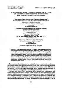
Flux linkage (Web.)
the simulation procedure is based on the data of the motor static characteristics. These characteristics include the flux linkage, co-energy and static torque curves where some of these curves are determined experimentally and others are completed analytically [13]. 2.1.1 Flux Linkage Current Curves Two flux linkage current curves at aligned and unaligned rotor positions are measured experimentally, and the intermediate curves are obtained analytically. Therefore, the vector of flux linkage can be obtained from the last estimated curves for any values of rotor position angle and stator current by interpolation if it lies between any two closest curves as shown in fig. (1). Then, all data are stored in a look-up table matrix i(θ, Ф). In this matrix, the current values are arranged such that the flux linkage values represent the row index and rotor position angles represent the column index as shown in fig. (2) [13].
2.2 Mechanical System The motor torque and speed will be affected by the sudden changes of operating point, so mechanical equations must be included for a complete modeling of SRM. The model of SRM for dynamic analysis consists of two sets of differential equations, the first one is the electrical differential equations (1) of the three phases, and the second is the mechanical differential equation described below [7]. dω 1 3 = [ ∑ τ j (θ j , i j ) − τ l − fω ] (2) dt J j =1 Where ω is angular speed, τl is load torque, f is viscose fraction coefficient and J is the inertia constant respectively. The system dynamics of SRM drives can be modeled as: ⎡ x&1 ⎤ ⎡0 − 1⎤ ⎡ x1 ⎤ ⎡0 ⎤ ⎡0 ⎤ (3) ⎢ x ⎥ + ⎢ ⎥ u + ⎢ ⎥ Tl ⎢ x& ⎥ = ⎢ ⎥ ⎣− b ⎦ ⎣ 2 ⎦ ⎣0 − a ⎦ ⎣ 2 ⎦ ⎣b⎦ Where a = f / J, b = 1 / J, x 1 = ωd - ω is speed error, ωd is desired reference speed, and x 2 = dω / dt. θ =45 o
θ =36 o
2
θ =24 o
Flux linkage (Web.)
θ =12 o θ =0 o
1.5
1
0.5
0
0
2
4
6
8
10
12
14
Current (Amp.)
Fig. (1) Flux linkage-current curves of 6/4 SRM.
ISBN: 978-988-17012-1-3
Fig. (2) 3D of flux, current, and position angle curves.
Static torque (N.m.)
2.1.2 Static Torque Curves Since, the phase static torque value illustrated in fig. (3) is obtained for any value of both current and rotor position angle. All data are stored in a look-up table matrix T(θ, i) by arranging the static torque values such that the current values give the row index, and the rotor position angles give the column index. Fig. (4) shows the block diagram of one phase for SRM.
Position (D eg.)
Current (Amp.)
Current (Amp.) Position angle (Deg.)
Fig. (3) 3D of static torque, current, and position curves. One phase block model θon
θoff
R
Inverter phase Vj switches and its θ logic
Vdc
on
Current table Torque table Look Look τj Фj up up 1/S Table ij Table Integrator i(θ, Ф) T(θ, i)
θoff θd
θj
θj Integrator ωref
1/S
θ
Periodicity
θ1
θj
Phase shifting ( j-1) θs
Fig. (4) The block diagram of one phase for SRM. 3. Control System 3.1 Sliding Mode Control If the speed error between the desired speed and actual rotor speed is: (4) x1 = e = ω d − ω Selecting the switching function (S). Since, the switching function is selected based on the system states as [4, 14]: (5) S ( x, t ) = (λe + e&) The design parameter (λ), which is the slope of the sliding line is selected such that (λ > 0) to ensure the asymptotic stability of the sliding mode [6]. Computing the time derivative for S (x, t), then (6) S& = λx& 1 + x& 2 To find the equivalent control law, put eqn. (6) equal to zero 1 u eq = [(λ + a) x 2 + cτ l ] (7) b The tracking problem ω = ωd can be considered as the state vector e remaining on the sliding surface S (x, t) = 0
IMECS 2008
Proceedings of the International MultiConference of Engineers and Computer Scientists 2008 Vol II IMECS 2008, 19-21 March, 2008, Hong Kong for all time. Lyapunov’s second method could be used to obtain the control law that would maintain this goal and a candidate function is defined as [4]: 1 V (S ) = S 2 (8) 2 It is aimed that the derivative of the Lyapunov function is negative definite. An efficient condition for the stability of the system described in eqn. (3) can be satisfied if one can assure that [5]: 1 d 2 V& ( S ) = S ≤ −η S , η ≥0 (9) 2 dt Obtaining the inequality in (9) means that the system is stable and controlled in such a way that the system states always move towards the sliding surface and hits it. Therefore, inequality (9) is called the reached condition for the sliding surface. Thus: S S& ≤ −η S or, (10) [−(λ + a) x 2 − cτ l ] sign( S ) +bu sign(S ) ≤ −η
(11) To achieve the sliding mode eqn. (8), the controller output must be chosen such that: u = u eq − K sign(S ) (12) To avoid the severe changes of the manipulated variable mentioned above, replace function sign(S) by sat(S) in eqn. (12). 3.2 Fuzzy Sliding Controller The combination between FLC and VSC is achieved to include their merits and avoid their disadvantages. This approach is used to implement fuzzy logic control based on variable structure technique which is called fuzzy sliding mode controller and applied for controlling the speed of SRM . Referring to the controller output of the VSC with sliding mode u stated in eqn. (12), which is expressed as equivalent control ueq and corrective control uc. (13) u = u eq + u c The proposed FSMC is divided into calculating equivalent control eqn. (7) and generating corrective control uc with fuzzy logic to maintain balance between robustness and chattering elimination. The process input state variables are chosen as: the error signal e between the actual and the desired speeds and the change in the error signal Δe. The fuzzy output variable is chosen as: the corrective control signal uc. 1 NB PB PS PM NM NS Z
cross the sliding surface on phase plane to satisfy existence condition. The control rules can be extracted from table (1). The min-max composition is chosen as a fuzzy inference method. Table 1: The rule data base for PI-like fuzzy controller. Δe, e NB NM NS Z PS PM PB NB NB NB NB NB NM NS Z NM NB NB NB NM NS Z PS NS NB NB NM NS Z PS PM Z NB NM NS Z PS PM PB PS NM NS Z PS PM PB PB PM NS Z PS PM PB PB PB PM Z PS PM PB PB PB PB 3.2.3 Defuzzification The output of the fuzzy controller is fuzzy sets, so it is necessary to convert these fuzzy sets to numerical values. Center of gravity (COG) algorithm is used to perform the defuzzification process. The selected membership functions of the output uc are seven symmetrical triangular shape as shown in fig. (5) . 4. Simulation Results The simulation study of the system, as shown in fig. (6), was implemented using matlab/simulink soft ware packages using the parameters of a typical three phase 6/4 pole SRM drive stated in reference [13]. The drive system is simulated with fixing the motor load and 1000 rpm constant reference speed. Fig. (7) shows the speed responses under using the proposed FSMC and PI controller. It is clear that the FSMC is better than PI controller in terms of all performance indexes. The motor speed traces the reference one when using FSMC without any overshoot and the settles faster than the PI controller. The total developed torque by the motor is shown in fig. (8) when applying FSMC. The controllers outputs are illustrated in fig. (9). Vdc limiter ωd
+
+
-
ω
ω
Applied voltage
-
FSMC
SRM
idc Fig. (6) Closed loop of SRM using proposed FSMC.
0.5
3.2.1 Fuzzification The error signal e and the change in error signal Δe are fuzzified using seven symmetrical triangular membership functions for simplicity. These membership functions are labeled NB, NM, NS, Z, PS, PM, and PB as shown in fig. (5). 3.2.2 Rule Evaluation The control rules must be designed such that the actual trajectory of the states always turns toward and does not
ISBN: 978-988-17012-1-3
Speed (r.p.m.)
0 0.5 1 1.5 0 -0.5 -1.5 -1 Fig. (5) MSFs of inputs and output variables.
1200 1000 800
Ref. speed
600
FSMC PI
400 200 0
0.15
0.3
0.45
0.6
0.75
0.9
1.05
1.2
1.35
1.5
Time (Sec.)
Fig. (7) Speed response with reference speed 1000 rpm.
IMECS 2008
Developed torque (N.m.)
Proceedings of the International MultiConference of Engineers and Computer Scientists 2008 Vol II IMECS 2008, 19-21 March, 2008, Hong Kong 1200
10
Speed (r.p.m.)
1000
8 6 4 2
800
Ref. speed
600
FSMC PI
400 200 0
0
0.3
0.6
0.9
1.2
Time (Sec.)
F
FSMC PI
6 3 0 0.6
0.9
1.2
0.5
1.5
0
0.5
Phase 1 voltage (V.)
330 220 110 0 -110 -220 2190
2220
2250
2280
1.5
2
2.5
3
F
ig. (14) Changing step load disterbance.
2310
2340
1200
Speed (r.p.m.)
The drive system is simulated with changing the speed reference step from 1000 to 400 rpm and again up to 1000 rpm and fixing the motor load as shown in fig. (13). It is observed that the motor speed response gives a good tracking for the reference one without overshooting under using the proposed controller.
2160
1
Time (Sec.)
The phase 1 excitation voltage, three phases instantaneous currents, and the total dc-link current via rotor position angle are shown in figures (10, 11, and 12) respectively, when using FSMC.
2130
3
1
Fig. (9) Fuzzy controller output.
2100
2.5
1.5
Time (Sec.)
-330 2070
2
Fig. (13) Motor speed and reference speed responses. Load step (N.m.)
Controllers outputs (Amp.)
9
0.3
1.5
2
12
0
1
Time (Sec.)
ig (8) Develoved motor torque.
-3
0.5
1.5
900 Ref. speed 600
FSMC PI
300 0
0.5
1
1.5
2
2.5
3
Time (Sec.)
Fig. (15) Speed responses with reference speed 900 rpm. The simulation is carried out using the FSMC and the PI controller when changing the load disturbance. The step load changing is shown in fig. (14). The speed responses of the motor are noted at reference speed 900 rpm as shown in fig. (15). It is clear that both the FSMC and the PI controller introduce excellent performance where the controlled variables track their reference values exactly in a very short time.
Position angle (Deg.)
Phases currents (Amp.)
Fig. (10) Phase1 voltage excitation. 3 2.5
i3
i2
i1
2
i3
i2
i1
i3
i2
i1
1.5 1 0.5 0 2070
2100
2130
2160
2190
2220
2250
2280
2310
2340
Position angle (Deg.)
3 2 1
800
0
700
-1 -2 -3 2070
2100
2130
2160
2190
2220
2250
2280
Position angle(Deg.)
Fig. (12) The total dc-link current.
2310
2340
Speed (r.p.m.)
Total dc–current (Amp.)
Fig. (11) Instantaneous three phases currents.
4.1 Sensitivity Analyses Sensitivity analyses are carried out to compare the dynamic performance of the system, using FSMC to some parameter variations of the motor. Considering 50% variation of significant system parameters such as moment of inertia coefficient, friction viscous coefficient, and motor phase resistance. Fig. (16) shows the speed responses with 600 rpm reference speed for the FSMC, when changing the inertia and friction coefficients. This figure indicates that, the system speed response is insensitive to the parameter variations when applying the FSMC. However, fig. (17) shows the speed responses but with varying the motor phase resistance by ±50% for 800 rpm reference speed. The performance response illustrates that the FSMC is more robust and insensitive to phases resistance variations. 600 500
Ref. speed 150% J, f 100% J, f 50% J, f
400 300 200 100 0
0.1
0.2
0.3
0.4
0.5
0.6
0.7
0.8
0.9
1
Time (Sec.)
ISBN: 978-988-17012-1-3
IMECS 2008
Proceedings of the International MultiConference of Engineers and Computer Scientists 2008 Vol II IMECS 2008, 19-21 March, 2008, Hong Kong Fig. (16) The speed responses with changing moment of inertia, and friction viscous coefficients using FSMC. Speed (r.p.m)
1000 800 Ref. speed 150% R 100% R 50% R
600 400 200 0
0.05
0.1
0.15
0.25
0.2
0.3
AND gates to produce the final chopped PWM full pulses for each power switch. Fig. (19) shows the chopped full pulses that are applied for the base-gate of the IGBTs power switches of the inverter. Fig. (20) illustrates the chopped voltage of one phase produced from the power inverter that is applied to one phase of the motor. The corresponding chopped phase current is shown in fig. (21). Finally, fig. (22) shows a typical step response using the proposed fuzzy sliding mode speed controller.
Time (Sec.)
Fig. (17) The speed responses with changing motor phase resistance using FSMC. Ch1
5. Experimental Results The closed loop control of SRM consists of an outer speed control loop and an inner current limitation control loop. The outer speed control loop is used to control the motor speed using the proposed FSMC. The actual rotor speed is obtained by estimating the rotor position angles through a software program, then it is compared with the reference command speed 900 rpm. By measuring the rotor position angles, the full switching signal patterns are generated. The speed error is processed through the proposed FSMC to produce a torque command. Form the torque command, the current reference command signal is obtained using the torque time constant. Consequently, the motor dc-link current is compared with the current command to get the current error. Then, this error is passed through a PWM circuit. Fig. (18) shows the practical output of the PWM circuit, where ch1 represents the triangular carrier signal with frequency of 3.3 KHz, ch2 represents the analog control signal (current error control signal) generated by the software, and ch3 shows the result of the instantaneous comparison between the two previous channels form of a logical train of pulses.
50 Volt/div.
Time
4 msec./div.
Fig. (20) Practical chopped phase voltage.
Ch1
Ch1
0.3 Amp./div.
Time
4 msec./div.
Fig. (21) Chopped phase current waveform.
Ch1
Ch1
Ch1
300 r.p.m./div.
Time
100 msec./div.
Fig. (22) Measured speed response of the motor.
Ch2
Ch3
Ch1
Ch1, 2, 3
2 Volt/div.
Time
100 µsec./div.
Fig. (18) Practical output of the PWM circuit. Ch1
Ch2 Ch3 Ch1, 2, 3
5 Volt/div.
Time
4 msec./div.
Fig. (19) The chopped phases gate pulses. The current error is compared with a triangular carrier with frequency (3.3 KHz) to generate the required pulse width modulation (PWM) control signal as channel 3 shows in fig. (18). These logical PWM trains of pulses, and the produced full switching signal pattern are passed through
ISBN: 978-988-17012-1-3
6. Conclusions This paper discusses the implementation of fuzzy sliding mode speed control for 6/4 poles SRM fed from classical inverter circuit. The paper visualizes both fuzzy logic control and variable structure control aspects, and definitions characterizing the fuzzy sliding mode controller. Full design procedure steps and its implementation of the proposed controller are obtained. Both simulation and experimental results are presented which show the validity and effectiveness of the proposed FSMC. The proposed fuzzy sliding mode controller, used for regulating the speed of SRM, has the following advantages: fast and smooth response, robustness, insensitivity to disturbance variations, and good tracking response. The closed loop speed control is achieved experimentally using the proposed FSMC. C-language program is used to simulate the FSMC to perform both read and write functions in addition to the controller simulation.
IMECS 2008
Proceedings of the International MultiConference of Engineers and Computer Scientists 2008 Vol II IMECS 2008, 19-21 March, 2008, Hong Kong Experimental results show flexibility of FSMC when used for speed control of SRM. 7. References [1] M. Spong, R. Marino, S.Peresada, and D.G. Taylor, “Feedback Linearizing Control of Switched Reluctance Motors” IEEE Trans. A.C. Contr., Vol. AC-32, pp. 371-379, May 1987. [2] R. S. Wallace, and D. G. Taylor, “A Balance Commutator for Switched Reluctance Motors to Reduce Torque Tipple”, IEEE Trans. Power Electron., Vol. 7, pp. 617-626, Oct. 1987. [3] R. Krishnan, “Switched Reluctance Motor Drives”, CDC press, 2001. [4] J. Slotine, and W. Li, “Applied Nonlinear Control” Englewood Cliffs, NJ: prentice Hall, 1991. [5] V. I. Utkin, “Variable Structure Control Systems with Sliding Mode” IEEE Trans. Automat. Contr., Vol. AC-22, pp. 210-222, April 1977. [6] J. Y. Hung, W. Gao, and J.C. Hung, “Variable Structure Control : A Survey” IEEE Trans. Ind. Electron., Vol. 40, No. 1, pp. 2-22, Feb. 1993. [7] K. D. Young, V. I. Utkin, U. Ozguner, “A Control Engineer’s Guide to Sliding Mode Control”, IEEE
ISBN: 978-988-17012-1-3
Trans. on Control Systems Technology, Vol. 7, No. 3, pp. 328-342, May 1999. [8] V. I. Utkin, “Sliding Mode in Control Optimization”, New York: Springer Verlag, 1992. [9] L. A. Zadeh, “Outline of a New Approach to Analysis of Complex Systems and Decision Process”, IEEE Trans. Sys., man, sybernetics, Vol. SMC-3, No. 1, pp. 28-44, Jan. 1973. [10] C. C. Lee, “Fuzzy Logic in Control Systems : Fuzzy Logic Controller, Part II”, IEEE Trans. on Systems, Man, and Cybernetics, Vol. 20, No. 2, pp. 419-435, March / April 1990. [11] G. Chen, T. Pham, J. Weiss, “Fuzzy Modeling of Control Systems”, IEEE Trans. on Aerospace and Electronic Systems, Vol. 31, No. 1, Jan. 1995. [12] D. Torrey, and J. Lang, “Modeling A Nonlinear Variable Reluctance Motor Drive”, IEE Proceedings , Pt. B, Vol. 137, No. 5, Sept. 1990. [13] M. Morsy, “Design and Implementation of Fuzzy Sliding Mode Controller for Switched Reluctance Motor”, PhD. Thesis, Egypt, Jan., 2007.
IMECS 2008