Based upon this identification process, a novel LabVIEW self-tuning PID controller is implemented in real time to control the response. The self-tuning controller ...
Page 0242
ISSN 2032-6653
The World Electric Vehicle Journal, Vol 2, Issue 4
Design and Implementation of On-Line Self-Tuning Control for PEM Fuel Cells Jonathan G. Williams*, Guo-Ping Liu*, Kary Thanapalan*, and David Rees* This paper presents the modelling and real time implementation of PEM (polymer electrolyte membrane) fuel cell flow control. Flow control presents a critical performance requirement to achieving dynamic power responses for electric vehicle motor demands. However a fuel cell’s complex structure and reactant requirements traditionally result in an unsatisfactory response to such dynamic loading instances. This in turn causes brief power losses associated with driving patterns such as acceleration and hill climbing. To improve the fuel cell’s dynamic response to such drive cycles, this paper presents new methodology for system identification and controller design. The fuel cell is modelled initially with established linear model and parameter estimation methods. The approach is then expanded to an on-line system identification LabVIEW programme to account for the non-linear and time varying characteristics. Based upon this identification process, a novel LabVIEW self-tuning PID controller is implemented in real time to control the response. The self-tuning controller continuously re-calculates the critical gain and period, and then adjusts the controller actions accordingly. Conclusions are then summarised from the results and future ongoing work is discussed briefly. Keywords: Fuel Cells, On-Line Identification, Non-Linear Dynamics, Time-Varying Systems, Self-Tuning Control the fuel cell stack. If the fuel cell is unable to respond adequately to large load variations, the continued voltage and power output drops associated to current inrushes of motors, results in momentary cell stress and drying of the membrane. Continued exposure weakens a cell, resulting in a low voltage output, which in turn increases the stresses on neighbouring cells in the stack, leading to a cascade failure and loss of the system.
1. INTRODUCTION The use of fuel cells as alternative power sources for mobile and stationary applications is steadily increasing as concerns over global oil reserves, escalating prices, and the environmental impacts of CO2 emissions increase. The dominant fuel cell technology for the automotive market is PEM (polymer electrolyte membrane). This is due to its compact design, favourable weight and power densities, along with low operating temperatures and quick start up times. PEM’s use of solid polymers also makes it favourable for ease of construction, and it exhibits good ability to respond to rapidly changing loads as experienced in automotive applications.
The complex, nonlinear dynamics of the fuel cell have been traditionally modelled using their approximated principles of electrochemistry, fluid dynamics, thermodynamics and heat transfer, in terms of the physical and material properties; along with universal constants under various assumptions and constraints. Earlier research work was focused on achieving steady state models of PEM fuel cells, describing the physical variables through Nernst equation, gas diffusion equation, and voltage drop and concentration equations. Recently there has been a noticeable increase in volume of dynamic subsystem research modelling of the transient response of PEM fuel cells. Pukrushpan et al. [1] is a noticeable contributor in this field, where he described the dynamics by a set of first order equations governing the air compressor, mass transportation and energy conservation of the reactant flows, and pressure across the anode and
This ability to respond to load changes depends on precise control of several subsystems. These include the temperature, humidity and pressure subsystems, which are closely associated to achieving final steady state value for a load request. Also, the reactant flow subsystem which is closely associated to the dynamic response to load changes, which is the focus of this research publication. The ability of the fuel cell to respond to dynamic loading instances is critical to the overall driver experience and life expectancy of *University of Glamorgan, Faculty of Advanced Technology, Pontypridd, Wales, UK CF37 1DL © 2008 WEV Journal
Design and Implementation of On-Line Self-Tuning Control for PEM Fuel Cells
7
Page 0243
ISSN 2032-6653
The World Electric Vehicle Journal, Vol 2, Issue 4
cathode. Cerola et al. [2] follows on providing more accurate partial differential equations to describe both the static and dynamic behaviours. Golbert and Lewin [3] constructed a spatial, time dependant fuel cell model covering the dynamics of water condensation on the electrodes, evaporation and generation. They also included a quasi steady state temperature profile. Pathapati et al [4] derived a dynamic model of the effects of the charge double layer capacitance and flow pressure dynamics, to allow predictions of the transient response of cell voltage temperature and gas flow rates under dynamically changing loads.
H2
O2
H2O
Cathode
Anode
H+ H2O H2O E-
Er Bip o la p la te
yer io n la
nel C ha n
D iffus
ye r on la
ye r on la
b ran e
ti Re ac
Mem
yer io n la
ti Re ac
D iffus
p la te
nel C ha n
r Bip o la
It is important to realise that no matter how complex the dynamic model, it never fully describes the fuel cell, and therefore system response, precisely in terms of system parameters. A fuel cell’s inherent nonlinearities and time varying characteristics inevitably pose difficult problems for system identification and control, making either linear or more complex nonlinear models, only valid over an operating range which exhibits linearity. Such models are typically used to investigate system stability, sensitivity, observability and controllability to allow controller designs. However if investigated in real time, these parameters with varying time operating states can be more closely identified to the system response with minimal error.
Figure 1: Fuel cell overview NA
Diffusion dynamics
Cathodic Kinetics
+
IC
+
R NH
Therefore, adaptive controllers can serve as a feedback law to achieve the control objectives with the time varying nonlinear properties, as well as external disturbances which is represented by factors such as loading of an electric vehicle motor. Previously referenced Pukrushpan et al. [1] implemented an observer based feedback controller to protect the stack from the previously described oxygen starvation effects during loading. This uses a linear quadratic technique based on a linearised state-space model. Other authors using such techniques to accommodate the nonlinearities include Paradkar et al. [5] who integrated a linearised PEM fuel cell model into a power plant, and simulated a load frequency controller. An optimal controller then accommodates the control application based on the disturbances. Schumacher et al. [6] deploy a fuzzy controller for the humidity management subsystem which adjusts the fan according to the requirement. Revenkar [7] highlights the requirement for further research into system models and controllers for multiple input, multiple output (MIMO) systems covering the whole operating range, a problem which is in part addressed within the proceeding sections.
Nernst equation
+
-
-
VC
Proton Concentration dynamics
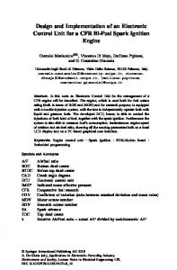
Figure 2: Fuel cell block diagram electrolyte, sandwiched between the anode and cathode electrodes. Each electrode then consists of a catalyst and gas diffusion layer to support the reaction which produces power and removes generated water. Figure 1 presents the structure of a PEM Fuel Cell. In order to develop a control strategy for a fuel cell’s flow, a model of the dynamic process is adopted from previous studies and described by its Nernst equation, anode and cathode gas diffusion, kinetics and proton concentration dynamics. From a system viewpoint, hydrogen is an input variable and is fed at an adjustable flow rate NH. Oxygen is also an input and can be represented by NA where a fuel cell uses the oxygen content of air. In the case of this publication, a compressed air cylinder fed via a regulated value is utilised for controllability. Voltage and Current are then considered the system outputs. Franklin et al
2. FUEL CELL MODELLING The referenced publications describe the fuel cell from its basic structure of a proton exchange membrane © 2008 WEV Journal
Oxygen
Hydrogen
Design and Implementation of On-Line Self-Tuning Control for PEM Fuel Cells
8
Page 0244
ISSN 2032-6653
The World Electric Vehicle Journal, Vol 2, Issue 4
[8] represents this as a standardised MIMO system represented by Figure 2.
2.1 Linear ARMAX Model Since the model of the fuel cell is very complicated, this paper focuses on the relationship between the oxygen flow and the voltage of the fuel cell. So hydrogen flow N H , is constant. The following ARMAX (autoregressive moving average with exogenous input) model in Equations (3), (4) and (5) is considered to describe the dynamics between the oxygen flow N A and voltage
From Figure 2, a standardised representation of the relationship can be formulated as shown in Figure 3, with blocks Gi , = 1,2,3,4, describing the relationship between the outputs I c and Vc , and inputs N A and N H , where R represents the internal cell resistance. Theoretically each block can then be linearised as its own transfer function describing its relationship. For example G1 represents the relationship between I c and N A . However, in practice this would be impossible to determine as blocks G2 , G3 , G4 would need to be eliminated to achieve a true representation, and the fuel cell cannot be sustained with only one reactant input. The overall stack model can be expressed as Equations (1) and (2).
Vc .
A( z −1 ) y ( K ) = Z − d B ( z −1 )u (k ) + w(k ) (3)
A( z −1) = 1 + a1 z −1 + a2 z −2 + ... + ag z −gγ γ
(4)
VC = G2 N A + G4 N H + R I IC
B( z −1) = b0 + b1 z −1 + b2 z −2 + ... + bbβ z −βb
(1)
(5)
I C = G1 N A + G3 N H
where y denotes the system output, u represents the system input, k denotes the time instant of sampling, and r and β are the order of A and B, respectively. w represents the constant disturbance of N A . Therefore without loss of generality a 0 = 1 . In descending order −1 part where z A z −1 y k defines the auto regression −h is the backward shift operator and z u (k ) represents −1 the past output. y k − h ; h = 1,2,...r ; B z u k denotes the moving average of past inputs, where z − h u (k ) = u (k − h) . Finally the corresponding transfer function between outputs and inputs in discrete form can be found as Equation (6).
(2) Equations (1) and (2) will now form the basis for the proceeding system identification methodology and design of a novel self-tuning PID controller programme and its application.
( )( )
(
G1
G ( z −1 ) =
IC
NA G2
−1
-
VC
G4
Figure 3: Approximated MIMO representation © 2008 WEV Journal
(6)
−1
Using linear theory all system modes can be excited using the ARXMAX approach by an impulse input signal of white noise. This has a frequency content entirely of sinusoidal waves of the same amplitude and strength, and can be generated with a pseudo random binary sequence (PRBS). However, in practice such an excitation signal could cause damage to the fuel cell in real time operation. The unit would not be able to respond to a PRBS large harmonic content, so instead a square wave excitation process would be implemented.
G3 +
( )( )
where A( z ) and B ( z ) are the polynomials given in Equations (4) and (5), respectively.
R
NH
B ( z −1 ) A( z −1 )
)
Design and Implementation of On-Line Self-Tuning Control for PEM Fuel Cells
9
Page 0245
ISSN 2032-6653
The World Electric Vehicle Journal, Vol 2, Issue 4
2.2 On-Line Parameter Estimation Expanding the ARXMAX identification methodology to include the recursive least squares algorithm (RLS), allows the identification process to predict the system output according to the past information. This allows for non-linear and time varying dynamics identification of the fuel cell. From Equations (3)-(5), the estimation of y (k ) is expressed as Equation (7)
›
yˆ (k ) = ϕf T (k − 1)qθˆ(k − 1) (7)
the characteristics of the system are unknown or time varying, as with fuel cells. The principle of adaptive control is to change the controller characteristics on the basis of the process change. Typically as with the self-tuning method utilised in this paper, the recursive identification processes is utilised. The task of on-line adaptive control is to maintain the optimal parameters of a difficulty to control process with time varying characteristics. This presents a complex process concisely explained in the following 3 step cyclic repetition. 1. The process parameters are assumed to be known for current control loop and equal to their current estimation.
where ϕf (k − 1) = [− y (k − 1), − y (k − 2),...,− y (k − γg), μu (k − d ), μu (k − d − 1),...,μu (k − d − βb ] (8)
2. The control strategy is designed based on the previous assumption and controller output is calculated.
(9)
3. The following identification step is performed after obtaining new controlled process variables. The parameters of the controlled process are recalculated using RLSM in this case (other Recursive methods can of course be utilised).
ϑJˆ T = [aˆ1 , aˆ 2 ,..., aˆγg , b0 , b1 ,..., bˆβb ]
After step k the new output is measured and a new set of parameters are obtained by Equations (10-12).
[
θqˆ(k ) = qθˆ(k − 1) + K (k ) y (k ) − f (k − 1)θqˆ(k − 1) ϕT
] (10)
[
K (k ) = P(k − 1)fθ(k − 1) × lλ + ϕf T (k − 1) P(k − 1)ϕf (k − 1)
]
−1
(11)
[
P (k ) = I − K (k )fϕ T (k − 1)
]P(kλl − 1)
(12)
where K (k ) is the estimation gain which brings the relative information of new measurements to update the parameter estimation. P (k ) is the covariance matrix which characterises the difference between the estimated and actual values where initially P (0) is chosen to be a large value. The coefficient lλ is called the forgetting factor which changes the importance of new information to old and has a range of 0 < lλ < 1. 3. CONTROLLER DESIGN Self-tuning controllers belong by their characteristics to the family of adaptive controllers. The aim of adaptive controllers is to solve control problems in cases where © 2008 WEV Journal
3.1 Digital PID Controllers Digital proportional integral derivative (PID) controllers remain widely accepted by industry due to their simplicity, convenience, and well known structures. Digital PID controllers use in fuel cell applications is extensively tried and accepted to give performance enhancements for an estimated model. However the non-linear and time varying characteristics of fuel cells mean the parameters are far from optimal, and require retuning over periods of operation. The adaptation of this well-known structure to a real time, self-tuning LabVIEW application is presented in proceeding sections, illustrating new methodology and material to this well understood controller. A generalised digital PID controller can therefore be derived from its continuous form given as Equation (13).
Gc ( s ) =
U (s) 1 = K p 1 + + Td s E (s) Ti s
(13)
where U (s ) is the process input, Y (s ) is the process output and E ( s ) = W ( s ) − Y ( s ) is the error where W (s ) is the reference signal. K p is the proportional gain, Ti is the integral and Td is the derivative action. The integral and derivative actions from Equation (13) are now discretised using the forward rectangular
Design and Implementation of On-Line Self-Tuning Control for PEM Fuel Cells
10
Page 0246
ISSN 2032-6653
The World Electric Vehicle Journal, Vol 2, Issue 4
method (FRM). In addition for on-line identification, the recursive control algorithm is incorporated to compute the actual controller value u (k ) from the previous value u (k − 1) and the compensation increment as Equation (14).
u (k ) = q0 e(k ) + q1e(k − 1) + q2 e(k − 2) + u (k − 1) (14) where the controller parameters are now Equation (15).
(
q0 , q1 , q3 = f K p , Ti , Td , T0
critical gain KPU, and ultimate period TU, using the work of Bobal et al and his book, “Digital Self Tuning Controllers” [9]. An overview of a generalised selftuning PID controller structure is presented in Figure 4. Bobal proposed the use of a discrete self-tuning method by considering a standardised single input, single output (SISO) system model in Equation (16).
G p ( z) =
)
(15) and T0 is the sampling period. 3.2 Design of Self-Tuning PID Control The Ziegler–Nichols methodology has been utilised throughout industry to determine both continuous and digital PID controller parameters. Similarly as with the generalised PID structure illustrated previously, its use in research does not present new material. However the following adaptation of the Ziegler–Nichols process of obtaining the proportional, integral, and derivative values does present new material and methodology. The process utilises a real time LabVIEW programme which identifies the ultimate parameters, known as
Y ( z ) z − d B( z −1 ) = U ( z) A( z −1 ) (16)
where U (z ) and Y (z ) are the z-transforms of the controller and process output, respectively. d denotes the time delay as integer T0 and A and B are the n - degree polynomials defined by Equation (4) and (5), respectively. So, let the process (17) be controlled by the proportional controller
GC ( z ) = U ( z )
E( z)
= KP (17)
where E ( z ) = W ( z ) − Y ( z ) is the transform of the control error, W (z ) is the z-transform of the reference signal.
Tuning parameters
Tuning Function
Performance Objectives
Disturbances
P + Setpoint + -
Error
I
+ +
Control effort
Process
Process variable
D Control function
Figure 4: Overview of self-tuning PID structure © 2008 WEV Journal
Design and Implementation of On-Line Self-Tuning Control for PEM Fuel Cells
11
Page 0247
ISSN 2032-6653
The World Electric Vehicle Journal, Vol 2, Issue 4
When solving (3) and (4) the following transfer function is obtained as Equation (20).
Gw ( z ) =
−d
START LABVIEW IDENTIIFCATION PROCESS
−1
z K p B( z ) Y ( z) = −1 W ( z ) A( z ) + z −d K p B ( z −1 )
(18)
where the denominator is termed as the characteristic equation for a closed loop.
D( z −1 ) = A( z −1 ) + z − d K p B ( z −1 )
K P1 =
1 − a2 b2
K P2 =
a1 − a2 − 1 b2 − b1
b = b1 K P1 + a1 c = b2 K P1 + a2
(19)
d = b 2 − 4c
Equation (19) can now be equated using the Unified Approach as utilised by Bobal for a 2nd order process as Equation (20).
a =−
b 2
TU (T0 ) =
2pT0 arccos a
D( z ) = z 2 + (a1 + b1 K P ) z + (a2 + b2 K P ) YES
(20) The approach presents two cases for identification of KPU and TU.
K PU = K P1
1. The critical poles lie on the real axis therefore the following equations (21) and (22) are valid for calculation of the critical values KPU and TU.
KPU PU (T0 ) =
a1 − a2 − 1 b2 − b1
d