Jul 25, 2012 - tion environment CASA (from version 3.4), and additional usage instructions can be found in the integrated help within CASA and in the CASA ...
ALMA Memo 593, 1–8; (2012)
Printed 26 July 2012
Design and Implementation of the wvrgcal Program B. Nikolic, S. F. Graves, R. C. Bolton and J. S. Richer Astrophysics Group, Cavendish Laboratory, Cambridge CB3 0HE, UK email: b. nikolic@ mrao. cam. ac. uk http: // www. mrao. cam. ac. uk/ ~ bn204/
arXiv:1207.6069v1 [astro-ph.IM] 25 Jul 2012
26 July 2012
ABSTRACT
This memo describes the software engineering and technical details of the design and implementation of the wvrgcal program and associated libraries. This program performs off-line correction of atmospheric phase fluctuations in ALMA observations, using the 183 GHz Water Vapour Radiometers (WVRs) installed on the ALMA 12 m dishes. The memo can be used as a guide for detailed study of the source code of the program for purposes of further development or maintenance. 1
INTRODUCTION
The ‘wvrgcal’ program is an application for off-line correction of atmospheric phase fluctuations in ALMA data based on observations of 183 GHz Water Vapour Radiometers (WVRs) that are installed on all ALMA 12 m-diameter antennas. The principles of WVR based phase correction, and of the algorithms used in ‘wvrgcal’ are described in previous papers and ALMA memos, e.g., Wiedner et al. (2001); Nikolic (2009); Nikolic et al. (2008), and forthcoming publications. In this memo we describe the technical details of the software engineering design and implementation of the wvrgcal program. This memo describes version 1.2 of wvrgcal which can be downloaded under the GNU Public License at http://www. mrao.cam.ac.uk/~bn204/soft. Brief usage instructions for astronomical users of wvrgcal can be found in the command line help (wvrgcal --help), shown in Appendix A. The program is currently shipped with the data reduction environment CASA (from version 3.4), and additional usage instructions can be found in the integrated help within CASA and in the CASA cookbook (http://casa.nrao.edu/ref_cookbook. shtml).
2
DESIGN
The phase correction process consists of four conceptual stages: (i) Computation of the phase correction coefficients. (ii) Use of the phase correction coefficients to transform the fluctuating sky temperatures into path estimates. (iii) Transformation of the path estimates to channel-specific phase corrections. (iv) Application of the phase correction to the astronomical visibility data. The wvrgcal program handles the first three stages of this process. The final stage is carried out similarly to the application of other calibrations – e.g. by using CASA or another interferometric data reduction package to apply the calibration table produced by wvrgcal. c 2012 The Authors
The design and control flow through the program consist of the first three stages, with a user-interface and control layer on top of them.
2.1
Initial processing of WVR data
Before the main phase correction steps are done, there is an initial pre-processing stage during which possible problems or artifacts are removed from the WVR data and optional smoothing is applied. Currently this processing consists of: (i) Filtering out measurements which may be affected by ALMA Calibration Arm blocking the WVR beam. (ii) Replacing data antennas with flagged WVRs or with no WVR at all with measurements interpolated from nearby antennas. (iii) Smoothing the WVR measurements in time. The filtering stage is carried out first to ensure that no averaging is done over data that may be contaminated. The filtering works on the basis of ‘scan intent’ of each of the measurements. Specifically, only WVR data marked with ON SOURCE and not marked with CALIBRATE ATMOSPHERE intents are kept and the remaining data are discarded. This process for example excludes any measurements when the ALMA Calibration Device (ACD) may have been moving (which can block or interfere with the WVR beam) or any sky-dip measurements of atmospheric transparency. The interpolation stage identifies the antennas that do not have a WVR (or have been flagged using --wvrflag). The WVR data for these antennas is replaced with a data-set interpolated from the three nearest antennas with un-flagged WVR data (see Sec.3.8). Smoothing of the WVR data is only carried out if the --smooth option is given, along with a specified number of time samples to smooth over. If it is requested, the smoothing process is carried out before any interpolation or filtering is performed. The smoothing process will not smooth across boundaries defined by the STATE ID flag.
2
Nikolic et al
Measurement Set
WV R
Ob
a nn te An
ser va
data
Smooth WVR Data WVR data
tio
nS
tat
Filtering WVR data
ns
io
sit po
e
Interpolation
tion rma info dow l win
WVR data
ctra
Spe
WVR data Select retrieval data
∼few WVR measurements dT /dL
Calculate path
Calculate dT /dL retrievals PWV, Bayesian evidence, dT /dL Feedback to user (to stdout)
Path estimates Scale Path estimates Convert to phase Phase estimates Write to CASA calibration table
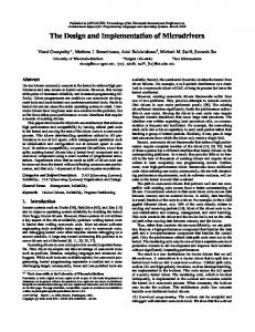
Figure 1. Flow of information within the wvrgcal program
2.2
Phase correction coefficient calculation
In the current version of wvrgcal, each set of phase correction coefficients is computed from a single integration (i.e., a single time point) of WVR data from a single antenna (an important investigation for the future is examining the differences between coefficients on different antennas or baselines). The absolute values of the WVR data from all four channels are used to best constrain the inference of properties of the atmosphere. These four values and the elevation of the antennas are currently the only information used in the inference – the ground level meteorological instrument data and oxygen sounder measurements are currently not used. Depending on the mode of operation of wvrgcal, one or more sets of phase correction coefficients may be computed for each observation. The mode of operation should be chosen by evaluating the likelihood that the optimal phase correction coefficient could have changed appreciably during observations. For example, if the observation being analysed consists of two sources at very different elevations, it is likely that the optimum phase correction coefficients will be different for the two sources, and at least two sets of coefficients should therefore be computed. The wvrgcal command line options which control the number of phase correction coefficient sets computed (and also how they are used) are: --nsol, --segsource and --tie. The --nsol option allows the user to specify directly the number of sets of phase correction coefficients that are to be computed.
These coefficients are always computed from the first antenna in the array, and with --nsol they are computed at time points evenly distributed in time over the observation. The --nsol option cannot be used together with the --segsource or --tie options. Since this option distributes the computation time points uniformly without particular regard to the sequence of the observation being analysed, it is usually useful only for very long tracks on a single object. Options --segsource and --tie, on the other hand, allow selection of when to recompute the phase correction coefficients based on the boundaries defined by the telescope moving to a new source. These two options are normally used in combination; furthermore, the option --tie cannot be used if --segsource is not also specified. The effect of the --segsource option is to specify that the phase correction coefficients should be re-computed each time the telescope moves to the next source. Here, source is used in the technical sense to mean the value in the “SOURCE” column in the data table. The explanation of option --tie needs to be divided into two stages, to prevent possible confusion in case of eventual further versions of wvrgcal: (i) Conceptually, the --tie option specifies to the wvrgcal program that best effort should be made to mutually accurately calibrate the phase of sources specified together after this command line option. In other words, the phase of these sources is “tied” together as best possible. 2012 ALMA Memo 593
WVRGCAL
3
(ii) In the current version of wvrgcal, this option in combination with --segsource is interpreted to mean that changes between sources in a “tie” group are not a trigger for re-calculation of the phase-correction coefficients. In other words, phase correction coefficients are re-calculated only when the telescope observations moves to a source which is not in the same tie group as the previous source.
Where:
Typical usage of this option is that science targets are “tied” together with their phase calibration sources, but not,for example, with the amplitude calibration sources. Regardless of which mode is used, the time points selected for computation are adjusted in the following way to maximise the appropriateness of the estimated coefficients:
When multiple sets of phase correction coefficients are used, the values of dTdLB,k to be used in equation 2 are always linearly interpolated in time between the two nearest sets of coefficients. Segments of time over which fixed coefficients are desired can be specified by entering the same coefficients at the beginning and end of the time segment – in this way the linear interpolation has no effect. This is the technique used when multiple coefficients are computed using the --segsource flag. At this stage, if any sources are flagged with --sourceflag, then the path estimates corresponding to the times when these sources were observed are set to zero. In this way no phase corrections for these sources is applied. This is useful when the observations of these particular sources are known to be corrupted, e.g., due to shadowing (one antenna blocking part of the field of view of another antenna). The next stage is to compute and provide some feedback to the user. This feedback consists of the RMS of the path fluctuation for each antenna and also the path ‘discrepancy’, which is described in Nikolic et al. (in prep). In order to make these statistics easier to interpret, the --statsource option can be used to compute the statistic for only a subset of the entire observation. When this option is selected, time intervals corresponding to the specified sources are computed and only the path estimates falling into these time intervals are used to compute the statistics. After computing the user feedback statistics, the estimated paths can be further scaled by using the --scale parameter. This parameter can be used to fine-tune the magnitude of the correction, but currently it is not recommended as the best way to use this has not been thoroughly studied. As the final part of the processing, the details of the spectral setup of the astronomical receivers is loaded and the computed path estimates are converted to a phase estimate. The conversion is carried out separately for each astronomical spectral window and channel, to take into account the changing wavelength. At this stage a dispersion correction can also be made (option --disperse), but this mode is also not commissioned and therefore not recommended for use.
• A time point near the middle of segment of time is selected to make the phase correction set as representative as possible. For example, if only one set of coefficients is calculated for an observation, then that set is computed from a time sample in the middle of the observation (and not at the beginning). • The scan intent of the data point is examined to ensure the telescope was not doing a calibration step at the time the datum was recorded. Once a WVR datum is selected for computation of the phase correction coefficients, it is passed (together with the telescope elevation) to a routine which does the computation using Bayesian model fitting. The technique used in the current version of wvrgcal is as described by Nikolic (2009), with an improvement in that Nested Sampling (Skilling 2006) is used instead of traditional MarkovChain Monte Carlo. The outputs of the Bayesian analysis are: • Probability distributions of the atmospheric water vapour column, pressure and temperature. • Probability distributions of the phase correction coefficients for each channel of the WVR. • A Bayesian evidence value, which measures how well the model describes the data. Currently the only quantities used for actual calibration are the mean values of the distributions of phase correction coefficients. The water vapour column, the estimated error and the Bayesian evidence are not directly used but are printed as feedback to the user. These quantities, as well as the estimated errors on the retrieved phase correction coefficients, could be used in the future to improve the phase correction performance – for example, by not using WVR channels for which the phase correction coefficients are poorly estimated. Once the phase correction coefficients are computed, they are used, together with the WVR data, to estimate the phase fluctuation for each antenna. In the standard mode of operation the path is computed as a weighted linear combination of the WVR brightness temperatures in the four channels: 4
∆L(t) =
∑ wk TB,k (t).
(1)
k=1
There is also an experimental (but not commissioned) mode of wvrgcal where the calculation is second order in path with respect to observed sky brightness. When a single set of phase correction coefficients is used for the whole observation, the weights are given by: !2 � � 1 dL 2 4 1 = δ TB,k (2) ∑ δ T dL . wk dTB,k i=1 B,i dTB,i 2012 ALMA Memo 593
dL: Final path estimate wk : The weight of the k-th channel TB,k : Observed brightness temperature of the k-th channel δ TB,k : Expected thermal-like noise in the k-th channel of WVRs dL dTB,k : Phase correction coefficient of the k-th channel
3 3.1
IMPLEMENTATION Build system
The compilation of the LibAIR package and the wvrgcal program is implemented using the standard GNU autoconf/automake build system. The benefits of this build system are: • Very high level of standardisation – the majority of GNU/Linux libraries and applications are built using this system. • Detection of features of the host system and checks for presence of prerequisite libraries. • Automatic dependency tracking for C/C++ programs. • Facilities for running unit-tests and creation of distribution tar-balls.
4
Nikolic et al
The configure script is generated from the configure.ac specification. The configure script takes a number of options that modify the way the LibAIR package is built. Some of the important options are:
Top-level src – main algorithms and computations apps – ALMA specific routines
--disable-pybind Do not try to build the Python binding. This option is recommended for all builds which are not intended for in-depth development of the library. --with-casa Location of the CASA package, which is required for building wvrgcal. The directory should point to the top of the CASA directory tree. --disable-buildtests Do not build the unit-tests – saves some time in compilation and removes the dependency on the Boost Unit Test library.
partitionsum testdata – Static partition sum data casawvr – binding to CASA mswvrdata – loading of WVR data msgaintable – write gain table information msantdata – load information about antennas cbind – Plain “C”-language binding cmdline – Command-line applications using libair
There are detailed worked examples on how to build the LibAIR library and all pre-requisites available at http://www.mrao.cam. ac.uk/~bn204/alma/sweng/libairbuild.html, and pages referred from there.
wvrgcal – main() for wvrgcal wvrretrieve – standalone pwv retrieval msdump – extract information from MS data
3.2
External Libraries
libair-ddefault – Dispersion data
The LibAIR package and wvrgcal program make use of a number of external libraries. The architecture, which is illustrated in Figure 2, has been designed to minimise cross-dependencies between nonstandard external libraries. Here is a short description of each of the external libraries: Boost Libraries: The Boost libraries are used for a variety of algorithms, containers and utilities throughout the package. They are a prerequisite for the entire LibAIR package and LibAIR can not be compiled without them. The Boost libraries can be downloaded from http://www.boost.org/. BNMin1: This is a minimisation/inference library. It is used to compute the Bayesian fit of the model to the observed atmospheric brightness in WVR channels. The library is available for download at http://www.mrao.cam.ac.uk/~bn204/oof/software.html. GNU Scientific Library (GSL): is a pre-requisite of BNMin1 package and is not used directly in LibAIR/wvrgcal. It is available for download from http://www.gnu.org/software/gsl/. HDF5: This is an optional input/output library for binary data. It is optionally used by wvrgcal, by the msdump program and for some testing/development purposes. The library is available for download from http://www.hdfgroup.org/downloads/. CASA: wvrgcal uses CASA (http://casa.nrao.edu/) libraries to read data from the input measurement set and write the gain calibration tables. Note that full CASA is required, not just casa-core SWIG The SWIG program and libraries are used to generate the Python-language bindings to the LibAIR. These bindings are in turn used only for development of the library and therefore SWIG is not required for compiling wvrgcal or other end-user tools. The SWIG program is available for download from http://www.swig.org/.
3.3
Directory Structure
The directory structure of the distributed source code is shown in Figure 3. The code is divided up into these directories depending on its intended functionality. The following sections describe the various aspects of LibAIR functionality, additionally mentioning where these can be found within the source code tree.
hd5wvr – HDF 5 I/O routines pybind – Binding to Python pyair.i – SWIG interface definition */all other files – Automatically generated test – Unit tests (based on Boost Test Framework)
Figure 3. Directory structure of the LibAIR source code
3.4
Command line parameter parsing
The parsing of command line parameters to the wvrgcal program is implemented using the Boost Program Options library (http://www.boost.org/doc/libs/release/libs/ program_options/). This is a widely used standard library for parsing command line options and is already used in some programs packaged with the CASA environment (e.g., the asdm2MS program). The listing of available command line options and a short description of each for wvrgcal are shown in Appendix A. These can be seen by executing wvrgcal --help.
3.5
Loading data from Measurement Sets
The wvrgcal program uses only the WVR data from the telescopes and does not require the astronomical auto- or cross-correlation data. As the volume of WVR data in all observations is very small it is feasible and convenient to load all of it into memory data structures for further processing. The memory data structure that is used is for storing this information is InterpArrayData which is declared in the file src/apps/arraydata.hpp. This data consists of simple linear arrays into which the relevant data from the MS are loaded. The arrays are ‘row-synchronous’, e.g., ith element of the time array is the timestamp of the ith element of the WVR data array. The loading itself, like all other code which needs to make use of casa-core or CASA libraries, is in the casawvr directory, primarily in mswvrdata.hpp. 2012 ALMA Memo 593
WVRGCAL
GSL
Boost
CASA
HDF5
BNMin1: inference / optimisation
LibAIR Core
LibAIR I/O for CASA
LibAIR I/O for HDF5
LibAIR Python bindings
wvrgcal: main userfacing application
msdump: Extract data from MS to HDF5
CASA dependent code
Better I/O
5
LibAir package SWIG
Core algorithms
Figure 2. Illustration of the software architecture of the wvrgcal program and supporting libraries.
3.6
Smoothing
If the command line option --smooth is called, then this smoothing of the WVR data is done before any other processing of the input data. If requested, this option replaces each WVR data point with a mean calculated within a smoothing window of the requested time width, and centred on that data point. If the number of samples to smooth over is an odd number, then the smoothing window is the requested width. If the number of samples (n) is an even number, then a smoothing window of n + 1 is used, and the first and last samples are only given 50% weight in the averaging. The smoothing process leaves unchanged WVR samples which are overly close to the start and end of the time range, such that there would not be sufficient data samples to fill the entire smoothing window. This process is performed by the function smoothWVR, defined within src/apps/arraydata.cpp.
3.7
Data filtering
The data filtering discussed in Sec. 2.1 (i.e. only data where the ‘scan intent’ is marked as ON SOURCE but not marked as CALIBRATE ATMOSPHERE are passed through). The identification of the correct data is done in the skyStateIDs function within casawvr/msutils.cpp. This information is passed by wvrgcal to the filtering function filterState, defined in src/apps/arraydata.cpp, which filters out unwanted data from further analysis. A similar process is used to filter out sources flagged by the user. A function filterInp is defined within cmdline/wvrgcal.cpp, and is called if the --sourceflag option is used; only samples whose source is not flagged are passed back out. This occurs just before the coefficient calculation is performed. 3.8
Interpolation
The interpolation of WVR data for antennas with no WVRs or with bad data is implemented in three stages: (i) Enumeration of antennas that need to be interpolated. This 2012 ALMA Memo 593
is done by parsing the --wvrflag command line option to get user-flagged antennas and calling the NoWVRAnts function (defined in cmdline/wvrgcal.cpp) to get automatically flagged antennas. NoWVRAnts currently automatically flags all antennas with names that begin with letters ‘CM’ (i.e., the compact array 7 m-diameter antennas, which do not have WVRs). (ii) Computation of nearest three antennas to each flagged antenna (excluding other flagged antennas) and the weight to be used (proportional to inverse distance) for each of the antennas (function linNearestAnt in file src/apps/antennautils.cpp) (iii) Replacing the data for bad antenna by the linear combination of data from the computed nearest antennas (function interpBadAntW in file src/apps/arraydata.cpp).
3.9
Atmospheric model
One of the key parts of the LibAIR package is the forward model for sky brightness around the 183 GHz water vapour line. This model is subsequently used for both the inference of the atmospheric properties and computation of the phase correction coefficients. The model is defined in files within the src/ directory. The physics of the model is described in Nikolic (2009). The implementation of the model is contained in files in the src subdirectory of the LibAIR distribution. The C++ code implementing the model is architectured as a polymorphic class hierarchy with the key functions being: • eval which computes the sky brightness in one channel or in all channels simultaneously • dTdc which computes the rate of change of sky brightness w.r.t. water vapour column These are declared in the base class WVRAtmoQuants in file model iface.hpp. The actual model used is made up by combining two classes: starting with a single layer water vapour model (class ISingleLayerWater declared in file singlelayerwater.hpp) and then adding model for the effect of zenith angle and imperfect coupling between WVR and sky (class CouplingModel in
6
Nikolic et al
model iface.hpp). Each component of the model declares its own parameters that are changeable at run time through the virtual function AddParams. 3.10
Implementation of retrieval of phase correction coefficients
After filtering and interpolation of the WVR data, wvrgcal next selects the individual time samples from which the phase correction coefficients are to be calculated. This selection is made by functions in the src/apps/almaabs.cpp file. If the --segsource option was supplied then the selection of time samples is done in function FieldMidPointI, which first calculates the range of times during which each set of separate sources (separated by function fieldSegmentsTied in src/apps/segmentation.cpp) was observed and then finds the mid point in time for each of these. Finally, it selects the next time sample after this midpoint which does not have a ‘bad’ (i.e., obscured by the ACD arm or not ON SOURCE) state. If the --segsource was not supplied, then a fixed number of coefficients, as selected by the --nsol option (default is 1), will be computed. The selection of data for this is done by function MultipleUniformI. This first finds equally spaced points over the full time range of the observation, and then selects the first sample after each of these time points which has a correct state (i.e. on source, and not performing atmospheric calibration). Both these functions for selecting data to compute phase correction coefficients will always take the data from the first antenna only (separate computation of coefficients for each antenna may be a useful eventual enhancement to the program). The selected data samples are stored within an ALMAAbsInpL structure, which is a list of ALMAAbsInput data objects (these are defined within src/apps/alma datastruct.h), one for each set of coefficients that will be calculated. These structures contain all the information used for phase correction coefficient calculation – the antenna number, WVR readings, elevation, time, state and source of the samples. The next step is the calculation of phase correction coefficients, which is triggered by the call to the function doALMAAbsRet (defined in file src/apps/almaabs.cpp). The inputs to this function are the selected WVR data, i.e., the ALMAAbsInpL structure described above. The function iterates through the ALMAAbsInpL, creating an object of class ALMAAbsRet from each datum, which itself creates an object of class iALMAAbsRet (defined within src/apps/almaabs i.cpp) and runs iALMAAbsRet::sample. This function sets-up and runs the nested sampler (using the class Minim::NestedS from the BNMin1 library). The nested sampler is specified to run for a maximum of 10000 samples – if the sampler is still making progress after this many samples a warning message is printed so that the user is aware that the sampler may not have fully converged. The results of the computation (i.e., the evidence, the precipitable water vapour and estimated error, and the dT dL coefficients for each WVR time datum) are printed to screen for each coefficient set. The coefficients are next converted into units of Kelvin/meter, and are used to compute the path correction for each antenna. These corrections are stored in an object of class ArrayGains (declared in src/almaabs/arraygains.hpp). This class, as well as calculating the path lengths/phase fluctuations required to create the gains within the output calibration table, also has various filtering, scaling and statistical functions.
If any sources were flagged by supplying the --sourceflag option, then the path correction estimates for these sources are set to zero in the function ArrayGain::blankSources. Subsequently, various statistics on the path lengths and the expected performance are calculated and printed to screen for the information of the user (see sec. 3.11, below). If the --scale option was supplied, then the path correction estimates are now uniformly scaled by the requested fraction, via ArrayGain::scale function. Finally, information about the spectral setup of the observation is loaded using the class MSSpec (declared in casawvr/msspec.hpp). The function loadspec defined in this file finds the frequency and channel information for each spectral window, using the casacore libraries to access these details. If the user has requested that the sign of the correction needs to be reversed for all the data (--reverse) or an individual spectral window (--reversespw) this is now changed within the output gains (using function reversedSPWS defined within cmdline/wvrgcal.cpp.
3.11
Computation of user feedback
The wvrgcal program outputs feedback to the user based on a statistical analysis of the WVR data recorded in the input Measurement Set. This feedback is mainly derived from the path length corrections computed previously for each antenna. The main part of the feedback is presented as a table with one row for each antenna in the dataset. This output consists of the number and the name of the antenna, if it contains WVR data, if it has been flagged with --wvrflag, the RMS of the path lengths for that antenna (in micron), and the discrepancy (Disc, also in units of micron). The RMS column shows the root-mean-square fluctuations of the computed path corrections, calculated in function ArrayGains::pathRMSAnt. Before computation of the RMS path fluctuation, the effect of the airmass is removed by multiplying the path corrections by sin θ where θ is the elevation of the antennas. The discrepancy column is computed in function computePathDisc in file cmdline/wvrgcal.cpp, which calls ArrayGains::pathDiscAnt . It is implemented by recalculating the phase coefficients so that firstly only the second channel is used, and then only the outermost channel is used. These coefficients are used to create two sets of estimates of the path corrections for the entire observation, which are then differenced. The RMS of the difference is computed. The sections of data used for computing these statistics can be controlled by using the command line option --statsource. By default the statistics are calculated using the data for the entire observation. However, the statistics can be computed only on one specific source by using the --statsource. For example, passing --statsource 1939-154 restricts the data used by the statistics computation to only those recorded while the antennas were on source 1939-154. The function statTimeMask in file cmdline/wvrgcal.cpp calculates the time ranges corresponding to the chosen source for the statistics calculation. The wvrgcal program also outputs expected performance of the calibration, which is computed in function printExpectedPerf in file cmdline/wvrgcal.cpp. The following values are computed: • The ‘thermal error’ – the expected RMS fluctuation in path corrections due to the intrinsic short-term noise in the mixers and amplifiers in the WVRs. This is computed in function thermal error (file src/apps/arraygains.cpp) and is based on the nominal 2012 ALMA Memo 593
WVRGCAL noise characteristics of the WVR channels, i.e., 0.1, 0.08, 0.08 and 0.09 K RMS channels 1 to 4 respectively. • The largest estimated path fluctuation on a single baseline, computed in function ArrayGains::greatestRMSBl by iterating through all baselines in the dataset, and for each of these computing the RMS of the difference between the phase corrections of the two antennas forming that baseline. • The estimated RMS path error due to the errors in the estimation of the phase correction coefficients. This is computed as the greatest estimated path fluctuation on a baseline (above), multiplied by the fractional coefficient error.
3.12
Dispersion correction
The wvrgcal program has an option to implement dispersion correction (--disperse). This option has not yet been commissioned and therefore is not recommended for use on science data. Curtis et al. (2009) showed that the dispersion correction is a very weak function of atmospheric conditions. Therefore, in the current version of wvrgcal, dispersion correction is implemented by interpolating a static table of correction as a function of frequency. This static table is stored in the data/libair-ddefault.csv file and is computed using the (A)ATM1 program. If this correction is requested, it is carried out within the function that writes out the final calibration table (writeNewGainTbl)
3.13
Output of Calibration Table
The output of the calibration tables is implemented in the file casawvr/msgaintable.cpp in function writeNewGainTbl (the name this function reflects the changes due to the update in the format of gain tables in version 3.4 of CASA). The implementation uses standard CASA C++ routines for creating and filling out calibration tables. The created calibration table has the phase correction information stored in the standard CPARAM column as a complex number (the amplitude of the correction is always unity as wvrgcal does not currently implement amplitude correction). If dispersion correction has been requested by supplying the --disperse parameter this function will also call the dispersion correction function before writing the phase corrections. When writing the calibration table the history sub-table is also populated with the exact command line invocation and version of wvrgcal used to generate it.
ACKNOWLEDGEMENTS This work was supported by the European Commission’s Sixth Framework Programme as part of the wider ‘Enhancement of Early ALMA Science’ project.
REFERENCES Curtis E. I., Nikolic B., Richer J. S., Pardo J. R., 2009, Atmospheric dispersion and the implications for phase calibration. ALMA Memo Series 590, The ALMA Project 1
Available from: www.mrao.cam.ac.uk/~bn204/alma/atmomodel. html 2012 ALMA Memo 593
7
Nikolic B., 2009, Inference of Coefficients for Use in Phase Correction I. ALMA Memo Series 587, The ALMA Project Nikolic B., Bolot R. C., Richer J. S., in prep, Quality Control of WVR Phase Correction Based on Differences Between WVR Channels. ALMA Memo Series in prep, The ALMA Project Nikolic B., Richer J., Hills R., Stirling A., 2008, Phase Correction for ALMA: Adaptive Optics in the Submillimetre. ESO Messenger 131, European Southern Observatory Skilling J., 2006, in ISBA 8th World Meeting on Bayesian Statistics Wiedner M. C., Hills R. E., Carlstrom J. E., Lay O. P., 2001, ApJ, 553, 1036
8
Nikolic et al
APPENDIX A: wvrgcal INLINE HELP AND COMMAND LINE OPTIONS WVRGCAL
-- Version 1.2
Developed by Bojan Nikolic at the University of Cambridge as part of EU FP6 ALMA Enhancement GPLv2 License -- you have a right to the source code (see http://www.mrao.cam.ac.uk/~bn204/alma) Write out a gain table based on WVR data GPL license -- you have the right to the source code. See COPYING Allowed options: --ms arg --output arg --toffset arg (=0) --nsol arg (=1) --help --segfield --segsource --reverse --reversespw arg --disperse --cont --wvrflag arg
--sourceflag arg --statfield arg --statsource arg --tie arg --smooth arg --scale arg (=1)
Input measurement set Name of the output file Time offset (in seconds) between interferometric and WVR data Number of solutions for phase correction coefficients to make during this observation Print information about program usage Do a new coefficient calculation for each field (this option is disabled, see segsource) Do a new coefficient calculation for each source Reverse the sign of correction in all SPW (e.g. due to AIV-1740) Reverse the sign correction for this spw Apply correction for dispersion UNTESTED! Estimate the continuum (e.g., due to clouds) Flag this WVR (labelled with either antenna number or antenna name) as bad, and replace its data with interpolated values Flag the WVR data for this source and do not produce any phase corrections on it Compute the statistics (Phase RMS, Disc) on this field only Compute the statistics (Phase RMS, Disc) on this source only Prioritise tieing the phase of these sources as well as possible Smooth WVR data by this many samples before applying the correction Scale the entire phase correction by this factor
2012 ALMA Memo 593