IOP PUBLISHING
PHYSICS IN MEDICINE AND BIOLOGY
Phys. Med. Biol. 55 (2010) 635–646
doi:10.1088/0031-9155/55/3/006
Design and initial performance of PlanTIS: a high-resolution positron emission tomograph for plants S Beer1,3 , M Streun1 , T Hombach2 , J Buehler2 , S Jahnke2 , M Khodaverdi1,4 , H Larue1 , S Minwuyelet2 , C Parl1 , G Roeb2 , U Schurr2 and K Ziemons1 1 2
Central Institute for Electronics, Forschungszentrum Juelich, D-52425 Juelich, Germany ICG-3: Phytosphere, Forschungszentrum Juelich, D-52425 Juelich, Germany
E-mail:
[email protected]
Received 20 October 2009, in final form 16 December 2009 Published 13 January 2010 Online at stacks.iop.org/PMB/55/635 Abstract Positron emitters such as 11C, 13N and 18F and their labelled compounds are widely used in clinical diagnosis and animal studies, but can also be used to study metabolic and physiological functions in plants dynamically and in vivo. A very particular tracer molecule is 11CO2 since it can be applied to a leaf as a gas. We have developed a Plant Tomographic Imaging System (PlanTIS), a high-resolution PET scanner for plant studies. Detectors, frontend electronics and data acquisition architecture of the scanner are based on the ClearPETTM system. The detectors consist of LSO and LuYAP crystals in phoswich configuration which are coupled to position-sensitive photomultiplier tubes. Signals are continuously sampled by free running ADCs, and data are stored in a list mode format. The detectors are arranged in a horizontal plane to allow the plants to be measured in the natural upright position. Two groups of four detector modules stand face-to-face and rotate around the field-of-view. This special system geometry requires dedicated image reconstruction and normalization procedures. We present the initial performance of the detector system and first phantom and plant measurements. (Some figures in this article are in colour only in the electronic version)
3 4
Simone Beer published under the name of Simone Weber until 2007. Maryam Khodaverdi is now at Philips Healthcare Germany, Aachen, Germany.
0031-9155/10/030635+12$30.00
© 2010 Institute of Physics and Engineering in Medicine
Printed in the UK
635
636
S Beer et al
1. Introduction Positron emission tomography (PET) is a non-invasive method for measuring molecular pathways and interactions in vivo. High-resolution PET systems dedicated for small animals such as mice and rats have found widespread use in pre-clinical research in the last decade (Chatziioannou 2002, Larobina et al 2006), but positron emitters such as 11C can be used for non-invasive studies of metabolism and physiological functions in plants as well (Ishioka et al 1999). The monitoring of radioactive-labelled molecules moving through a plant has been performed so far by autoradiography, or by collimated or coincident gamma detectors placed at leaves, stems or other plant organs (Minchin and Thorpe 2003, Thorpe et al 2007, Jaeger et al 1988). The count rates provide the time behaviour of radioactivity in the corresponding parts of the plant. Much more detailed information is obtained by a planar camera such as the Duke VIPER (Kiser et al 2008) which is optionally combined with coincidence counting as a hybrid system, or the PETIS (Positron Emitting Tracer Imaging System) which has been used to analyse e.g. carbon kinetics during photosynthesis in a leaf using a compartment model (Kawachi et al 2006). Complex plant organs such as fruits or the root system within the soil make tomographic imaging necessary in order to get the full three-dimensional information. Hence, we have developed a PET scanner designed as a Plant Tomographic Imaging System (PlanTIS). With this scanner, the factors determining the allocation of carbon to different plant organs, one of the grand challenges of modern plant biology, can be studied non-invasively and in closeto-natural conditions. In combination with MRI, plant structures and transport processes can be analysed, in relation to genomic, developmental or environmental challenges (Jahnke et al 2009). 2. Description of the system 2.1. Detectors The data acquisition system and the detectors widely correspond to those of the ClearPETTM system (Ziemons et al 2005, Streun et al 2006). The detectors consist of multichannel photomultiplier tubes (H7600-00-M64, Hamamatsu), each of them reading out 64 scintillator pixels (figure 1(a)). A single pixel is a phoswich arrangement of an LSO and a LuYAP (Kuntner et al 2005, Weber et al 2003) crystal which can give depth of interaction information (DOI). Each pixel is directly coupled to one photomultiplier channel. The crystals are polished and encapsulated in BaSO4 matrices for mechanical stability and to increase light output. The strong gain variation of the photomultiplier channels is equalized by a mask with a hole of individual size above the light entrance of each channel (Christ et al 2003). Hence, not only the anode signals but also the signal at the last dynode of the photomultiplier is corrected, which is used for the determination of arrival time, energy and pulse shape. The relative light transmission of the holes varies between 100% and 36%. A similar mask but with identical hole sizes is placed between the LSO and LuYAP crystal layers. It reduces the light intensity of the LSO layer to 64% in order to match the higher light output of LSO to that of LuYAP. Unfortunately, the size of the photomultiplier is larger than its sensitive area. This results in gaps between the crystal matrices of adjacent detectors. The gaps can be avoided by using optical fibres as light guides between crystals and photomultiplier (Cherry et al 1997), but the drawback for PlanTIS was the further loss of light which could not be accepted.
Design and initial performance of PlanTIS, a high resolution PET for plants
637
Figure 1. (a) Detector head, consisting of two layers with 64 LSO and LuYAP crystals in the phoswich configuration. (b) PlanTIS system: four detector modules, consisting of four detectors each, stand face-to-face and rotate around the field-of-view. Every second module is shifted axially to cover the axial gaps during rotation.
2.2. General design The PlanTIS system is equipped with eight modules consisting of four detectors each, which are arranged in parts of a ring so that four modules on one side are diametrically facing the other four modules (figure 1(b)). The gaps between the crystal matrices cause insensitive regions between the detectors axially and tangentially. Every other module is therefore shifted vertically by 9.2 mm, and because the scanner rotates in a horizontal plane both the axial and the transaxial gaps are covered. PlanTIS has an axial field-of-view (FOV) of 10.1 cm and a transaxial FOV of 7.3 cm. The detectors are assembled on a table, and plants can be placed in such a way that the parts of interest reach through a hole in the table top into the field of view. Scans are performed in continuous mode, i.e. data are recorded continuously during a full 360◦ rotation. One full rotation can be completed in 30 s. Due to the symmetric detector arrangement, dynamic studies can be realized with a time frame period of 15 s. 2.3. Data acquisition A trigger signal from one of the photomultiplier channels indicates the occurrence and position of a scintillation event. The analogue pulse at the dynode of the photomultiplier is digitized by a free running ADC (analogue to digital converter). For each registered event, a data package is generated containing the position, the sampled pulse and a time stamp (Streun et al 2006). The time stamp is obtained from a counter in the detector module. The counters in all the detector modules run synchronously due to a central clock and reset unit. These data are sent via optical fibre to one of two preprocessing PCs which are connected by a local network to a master PC and a file server. The master PC controls the whole scanning process, while the file server receives the preprocessed data from the preprocessing PCs and stores them on a fast hard disk system. Usually, all single events are stored and coincidence detection is performed offline using the time stamp in the event data. The PlanTIS system provides the additional option of a hardware coincidence circuit between the detector blocks. When activated, the detector modules register only events which are approximately simultaneous in both blocks. The principle of this circuit is shown in figure 2. Within each detector module, trigger signals
638
S Beer et al
Figure 2. Detector module with coincidence circuit. The trigger outputs of the four modules of one detector group are directly connected and form a wired OR gate. This signal is the trigger input for all modules of the opposing group.
from the photomultiplier can initiate the recording of the event only if a trigger signal was received from one of the opposite detector blocks. The time window is rather wide (∼100 ns), and the circuit is not supposed to replace the offline coincidence detection but is effective in data reduction. The wide hardware window allows also the use of a delayed window technique for the estimation of random coincidences. A lower energy threshold can be applied by software during acquisition. In general it is set to 350 keV. The upper threshold is fixed to 1280 keV. The data are stored in a dedicated listmode format which is able to handle data from both singles and coincidence data (Weber et al 2006). Each event can not only be described by the respective detector IDs and energies but other information can also be coded, such as time information or position of gantry and source. A timing window of 25 ns is applied. The coincidence data are binned into 3D sinograms for reconstruction. The sinograms have 65 tangential bins and 180 angular bins. The ring difference is indexed by segments, and for all measurements 31 segments are used (Weber et al 2006). No axial compression is applied. 2.4. Data correction The gaps between the detectors were accepted on the one hand because manufacturing of the detectors is easier, on the other hand to avoid a potential decrease of light output due to light guides additionally to the light loss due to the masks. However, it is crucial to apply adequate data corrections before image reconstruction if artefacts are to be avoided. Normalization factors can be described as a product of various normalization components, namely the intrinsic crystal efficiency, the general geometry of the system and a ‘crystal interference factor’ (Casey et al 1995). The crystal interference refers to the differences between detection efficiencies of crystals due to shielding by neighbours, or by the first layer in the case of phoswich detectors, and crystals at the border of detectors which have no neighbours and are hence unshielded. In comparison to ring scanners, the relative importance of the correction factors change, and the most important correction for PlanTIS is the normalization of the scanner geometry, followed by the correction of crystal interference and the correction of individual detector efficiencies (Weber et al 2005). The individual detector efficiencies are of minor relevance since the detectors are rotating, so that the efficiencies are averaged. The tracer we have used so far is 11C, with a half life of only 20.4 min. Measurements over several half lives are standard, starting with high initial activity. Therefore, adequate dead time correction is necessary.
Design and initial performance of PlanTIS, a high resolution PET for plants
639
Figure 3. Due to the axial and transaxial gaps of the scanner, the sinograms show a typical structure. Direct sinograms (a), and their projections (b), of a large cylinder in a ring where, due to the axial shift of every second module, only half of the modules contribute (3, top) and in a ring where all modules contribute (4, bottom).
2.4.1. Normalization of geometric sensitivity. For each ring difference, two configurations are possible: (a) rings where all eight modules contribute to the data, and (b) rings where only every second module contributes due to the axial shift of the detectors. For PlanTIS, we have e.g. 48 direct sinograms, from which 16 are composed of rings where all modules contribute, and 32 are composed of rings where every second module contributes. Figure 3 shows an example of a sinogram of a large cylinder for both sinogram types, together with projections of the sinograms, summed over all angles. The sinograms’ strip pattern, strong in case (b), and moderate in case (a), needs to be corrected during the iterative image reconstruction (Weber et al 2006) (see section 2.5). 2.4.2. Normalization of crystal interference and detector efficiencies. We measure the normalization factors of both crystal interference and detector inhomogeneities using a cylinder, homogeneously filled with 11C in water, with an inner diameter of 69 mm to cover a large part of the FOV. Precise centring of the cylinder remains ensured mechanically by means of centring rings. The data are binned into sinograms and corrected for both attenuation and the amount of activity between two crystals using sinograms of a mathematical cylinder with the same dimensions. The corrected sinograms are then averaged over all angles. This saves measurement time and is reasonable because, due to the scanner rotation, crystal efficiencies are averaged anyway. Finally, the sinograms are simply backprojected into an image which is used as a sensitivity image within the iterative reconstruction. 2.4.3. Dead time correction. For the estimation of dead time correction factors we use a cylindrical phantom, containing a high initial 11C activity solution. Data are acquired over several half lives and are merged into frames of 5 min duration. The count rate data are then fitted using the dead time model Rmeas = aRtrue exp(−bRtrue ) + offset
640
S Beer et al
for each detector after correction for random coincidences. Dead time correction factors are then calculated for each detector as the ratio of measured counts and the linear interpolation of the fit in the region of low activity where no dead time occurs. An overall dead time correction factor is applied to the measured data by estimating the count rate and dead time correction factor for each detector, and weighting the correction factors according to the amount of data from the respective detector. 2.5. Image reconstruction Based on the corrected 3D sinograms, the data are reconstructed using a fully 3D ‘ordered subset a posteriori one-step late’ (OSMAPOSL) algorithm. The algorithm is based on ‘Software for Tomographic Image Reconstruction’ (STIR),5 an object-oriented Open Source software consisting of classes, functions and utilities for 3D PET image reconstruction (Labb´e et al 1999a, 1999b). It allows zooming the application of inter-update, inter-iteration or post-filtering and the application of prior information in an additive or multiplicative way. Due to the above-mentioned strip pattern of the sinograms, a straightforward application of STIR-OSEM yields to severe image artefacts. All supported algorithms require a precomputation of the sensitivity image of the scanner. We do not use the STIR implementation for the pre-computation of the sensitivity image, but use the backprojected data of the normalization measurement, which comes with the geometric sensitivity included. Unless otherwise noted, we run the algorithm as Ordered-Subset ExpectationMaximization (OSEM) without any filtering or prior information, with 5 subsets and 20 subiterations. 2.6.
11
CO2 labelling of plants
11
CO2 is produced by a cyclotron (Japanese Steel BC 1710) of the Institute of Nuclear Chemistry (INM-5) located near the facilities for plant experiments. The radioactive gas is administered to the plants by an 11CO2 application system. The apical parts of leaves are clamped in a transparent leaf cuvette and labelling is performed by injecting the radioactive gas into the gas line connecting the application system with the cuvette. Anything from a short pulse to a continuous supply can be used, depending on the application. After administering 11 CO2, the system is opened and the radioactive gas replaced by normal air. Similar to inactive 12 CO2, radioactive 11CO2 is taken up by the leaves via photosynthesis by which so-called photoassimilates are produced. Some photoassimilates may (temporarily) stay in the leaves while others are allocated to plant parts which demand organic carbon (in particular growing regions of a plant). The 11C-labelled fraction of photoassimilates transported e.g. to the roots may become detected and imaged by using PlanTIS. 3. Results 3.1. Initial performance 3.1.1. Time resolution. The homogeneously 11C-filled normalization cylinder was scanned for 200 min with the hardware coincidence activated. The time difference between two coincident events is recorded. Figure 4 shows the respective timing histogram. The true coincidences form a sharp peak which stands on a base of random coincidences. The FWHM, estimated by a Gauss fit to the peak, is 12.4 ns. The intrinsically good timing resolution of 5
http://stir.sourceforge.net.
Design and initial performance of PlanTIS, a high resolution PET for plants
641
Figure 4. Timing histogram with activated hardware coincidence.
the scintillators cannot fully be exploited due to the light attenuating masks in the detector heads. 3.1.2. Intrinsic spatial resolution. The intrinsic resolution was measured with an 18F line source with an inner diameter of 1 mm. The source was placed near the centre of field of view and moved in 0.5 mm steps in the radial direction perpendicular to an opposing pair of detector modules. The coincident count distribution detected by each pair of opposing crystals in these modules was fitted with a Gaussian function to determine the intrinsic resolution. The average measured FWHM was 1.48 mm, without correction for the source dimension. 3.1.3. Spatial resolution and effect of DOI. The spatial resolution was measured using a 22Na point source with 0.25 mm active diameter of 415 kBq, encapsulated in a 1 × 1 × 1cm3 acrylic cube. The point source was positioned in the centre of the FOV and at 5 mm, 10 mm, 15 mm and 25 mm off-centre. The lower energy threshold was set to 350 keV. The maximum random coincidence rate was less than 3.6%. At least 2 × 10⁶ prompts were acquired at each position. The data were reconstructed using the OSEM algorithm with a zoom factor of 5, resulting in an image matrix with 323 × 323 × 95 voxels and a voxel size of 0.23 mm × 0.23 mm × 1.15 mm. Response functions through the peak of the image were created by summing all one-dimensional profiles that are parallel to the direction of measurement within at least two times the expected FWHM of the orthogonal directions. For radial and tangential resolutions, the maximum values were determined by a parabolic fit using the peak point and the nearest one or two neighbours. The FWHM and FWTM were determined by linear interpolation between adjacent pixels at half and one-tenth the maximum values of the response function. Axial resolutions could not be determined in this way because the zooming was not applied to the slice thickness, but were calculated by a gauss fit. The radial, tangential and axial resolutions (FWHM) at the centre of the FOV were 1.39 mm, 1.26 mm and 1.45 mm, respectively. At a radial offset of 25 mm, the FWHM values were 2.31 mm, 1.88 mm and 1.46 mm. When the DOI information is ignored, the radial resolution at 25 mm deteriorates to 2.76 mm. Figure 5 shows the radial (with and without DOI), tangential and axial FWHM and FWTM as a function of radial offset.
642
S Beer et al
Figure 5. Radial, tangential and axial FWHM and FWTM of the PlanTIS scanner versus radial offset. The radial resolution was determined with and without DOI information.
Figure 6. Slices of a homogeneously filled cylinder phantom (69 mm Ø) after normalization of geometry, crystal interference and detector efficiencies as well as attenuation correction. Except for the early slices (upper left corner), the images show an acceptable homogeneity.
3.1.4. Peak sensitivity. The peak sensitivity was measured using the same point source as for the spatial resolution measurement. The source was positioned in the centre of the scanner and was scanned for 3.5 min. The peak sensitivity in the centre of the scanner amounts to 3.7%. 3.1.5. Homogeneity. Figure 6 shows different slices of the reconstructed image of a cylinder with an inner diameter of 69 mm which was homogeneously filled with an aqueous 11Ccarbonate solution. Besides the normalization procedure, the data were corrected for attenuation using a calculated attenuation correction based on a mathematical cylinder phantom. The standard deviation within a central region-of-interest (ROI) of 51 mm diameter (∼75% of the cylinder diameter) and 10 mm axial extent is 5.4%. Within an ROI of the same diameter and an axial extent of 71 mm (∼75% of the cylinder length), the standard deviation is 5.8%.
Design and initial performance of PlanTIS, a high resolution PET for plants
643
Figure 7. ROI average with and without dead time correction for time frames of a homogeneous cylinder within a central ROI of ∼75% of the cylinder diameter. Logarithmic scale.
Figure 8. Central slice of a Micro Deluxe phantom (Data Spectrum Corp.) with an inner diameter of 4.5 cm and hollow channel diameters of 1.2, 1.6, 2.4, 3.2, 4.0 and 4.8 mm.
3.1.6. Dead time correction. The same 69 mm diameter cylinder, filled with 11C-carbonate in water, was scanned over several half lives. The data were binned into frames of 5 min duration. During data reconstruction only geometrical as well as detector normalization has been applied, but no correction for e.g. scatter. Figure 7 shows the ROI average for several time frames within a central ROI of 51 mm diameter, with and without dead time correction and the respective exponential decay. 3.2. Phantom images A Micro Deluxe phantom (Data Spectrum Corp.) with an inner diameter of 4.5 cm and hollow channel diameters of 1.2, 1.6, 2.4, 3.2, 4.0 and 4.8 mm was filled with 11C-carbonate in water and scanned for 30 min. The centre-to-centre spacing of the rods is equal to twice the rod diameter. The lower energy threshold was set to 350 keV. The data were corrected for random coincidences and reconstructed using the OSEM algorithm with 5 subsets and 60 subiterations. No zooming was applied, which results in a pixel size of 1.15 mm × 1.15 mm. A reconstructed transverse slice of the phantom is shown in figure 8. The rods with 2.4 mm diameter are clearly separated. The separation of the 1.6 mm rods suffers from the limits in spatial resolution off-centre as well as positron range of 11C and partial volume effects, so they are barely distinguishable.
644
S Beer et al
Figure 9. PET scan of a barley root in soil after 11C application to the leafs.
3.3. Plant images A barley (Hordeum vulgare) plant was positioned with the roots, growing in soil, in the field of view of PlanTIS. The upper 3.5 cm of the older leaf was clamped in the leaf cuvette about 12.6 cm above the root pot and 11CO2 was administered for a 26 min long pulse, starting with an initial activity of 244 MBq. Data were acquired for 150 min and binned into time frames of 5 min duration. Besides normalization of geometry and detector inhomogeneities, no further corrections were applied. Figure 9 shows the image of a 5 min time frame, containing 6 × 10⁵ counts, using volume rendering. The overall length of the root is 6.4 cm; distinct parts of the roots such as root tips are visible. 4. Discussion Plants are highly dynamic organisms which are often exposed to varying environmental conditions without the ability to avoid harmful environments by moving away. A central goal of plant science is to understand the regulatory mechanisms of plant growth in a changing environment. Plant tissues such as phloem (a pathway for the transfer of carbohydrates from their site of synthesis in leaves to the sites of utilization, e.g. roots) and xylem (the pathway for transport of water and mineral ions from the soil) form a highly developed vascular network which is not only responsible for transport processes but acts also as a signalling network coordinating the organ functions. Physical access to the transport system for any measurements is extremely problematic. For example, phloem tissues have high hydrostatic pressures (Gould et al 2004) and are extremely sensitive to manipulation, and xylem tissues are vulnerable because of very low pressures. It is vital therefore to use non-invasive techniques, such as high-resolution PET, in order to study the function of these systems. Besides 11C, other short-lived positron-emitting isotopes such as 13N, 15O and 18F can be used to label biologically active molecules, nutrients or compounds which are absorbed via normal metabolism and distributed throughout the plant (Kiser et al 2008).
Design and initial performance of PlanTIS, a high resolution PET for plants
645
First data analysis techniques such as compartmental analysis (Fares et al 1988) or the input-output-model (Minchin 1978) have been used in studies where 11C transport was measured using collimated detectors, but are under discussion (Minchin and Thorpe 2003). Since a successful tracer kinetic model is a blend of physiology, instrumentation, statistics, mathematics and practical logistics (Carson 1991), the development of advanced model formulation and methodology will profit from the better spatial information of tracer distribution in 3D image data, especially as it allows the regions of interest to be specified after data are collected. With collimated detectors such freedom is not possible. We have developed a high-resolution PET scanner dedicated to plant imaging, based on technology which is used for small-animal PET. With its spatial resolution of ∼1.4 mm in the centre, a peak sensitivity of 3.7%, a FOV diameter of 7.3 cm and an axial FOV of ∼10 cm, the scanner can be used for a variety of applications in plant science. Nevertheless, there will be several challenges when PET technology is used for this kind of application. For example, radiotracer transport and the allocation of the tracer within the plant proceed over long periods of time. Due to the short half life of 11C, the dynamic phenomena which can be observed are limited to those with characteristic time constants of only a few hours, which means a high initial activity is necessary, for measurements over many half lives. Tracer in the plant is often close to the surface, be it moving or stationary. The amount of surrounding tissue can therefore be very thin so that some positrons will escape and travel some distance in air before annihilation. Nevertheless, some material can be placed near the surface of the plant to ensure annihilation occurs there (Minchin and Thorpe 2003). Another challenge can be radiation scattered from the highly radioactive region where 11CO2 gas is applied, which can be just outside the edge of the field-of-view. PET itself is multi-disciplinary, with scanner design and the methodology of PET measurements being highly application-dependent. This is of special importance when a new application such as plant PET is considered. Collaborative research and a good teamwork among all disciplines, from chemistry, engineering and mathematics to biology and plant physiology, covering all parts of a PET study, are required to make effective use of this technique. Acknowledgments We thank Marco Dautzenberg for laboratory assistance, and Dr Michael Thorpe for very useful comments on this manuscript. References Carson R E 1991 The development and application of mathematical models in nuclear medicine [editorial] J. Nucl. Med. 32 2206–8 Casey M E, Gadagkar H and Newport D 1995 A component based method for normalization in volume PET Proc. 3rd Int. Meeting on Fully Three-Dimensional Image Reconstruction in Radiology and Nuclear Medicine (Aix-les-Bains, France) pp 67–71 Chatziioannou A 2002 Molecular imaging of small animals with dedicated PET tomographs Eur. J. Nucl. Med. 29 98–114 Cherry S R et al 1997 MicroPET: a high resolution PET scanner for imaging small animals IEEE Trans. Nucl. Sci. 44 1161–6 Christ D, Hollendung A, Larue H, Parl C, Streun M, Weber S, Ziemons K and Halling H 2003 Homogenization of the multichannel PM gain by inserting light attenuating masks IEEE Nucl. Sci. Symp. Conf. Record 4 2382–5 Fares Y, Goeschl J D, Magnuson C E, Scheld H W and Strain B R 1988 Tracer kinetics of plants carbon allocation with continuously produced 11CO2 J. Radioanal. Nucl. Chem. 124 105–22
646
S Beer et al
Gould N, Minchin P E H and Thorpe M R 2004 Direct measurements of sieve element hydrostatic pressure reveal strong regulation after pathway blockage Funct. Plant Biol. 31 987–93 Ishioka N S et al 1999 Production of positron emitters and application of their labeled compounds to plant studies J. Radioanal. Nucl. Chem. 239 417–21 Jaeger C H, Goeschl J D, Magnuson C E, Fares Y and Strain B R 1988 Short-term responses of phloem transport to mechanical perturbation Physiol. Plant 72 588–94 Jahnke S et al 2009 Combined MRI-PET dissects dynamic changes in plant structures and functions Plant J. 59 634–44 Kawachi N, Sakamoto K, Ishii S, Fujimaki S, Suzui N, Ishioka N S and Matsuhashi S 2006 Kinetic analysis of carbon-11-labeled carbon dioxide for studying photosynthesis in a leaf using Positron Emitting Tracer Imaging System IEEE Trans. Nucl. Sci. 53 2991–7 Kiser M R, Reid C D, Crowell A S, Phillips R P and Howell C R 2008 Exploring the transport of plant metabolites using positron emitting radiotracers HFSP J. 2 189–204 Kuntner C, Auffray E, Bellotto D, Dujardin C, Grumbach N, Kamenskikh I A, Lecoq P, Mojzisova H, Pedrini C and Schneegans M 2005 Advances in the scintillation performance of LuYAP:Ce single crystals Nucl. Instrum. Methods A 537 295–301 Labb´e C et al 1999a An object-oriented library for 3D PET reconstruction using parallel computing Proc. of Bildverarbeitung fuer die Medizin 1999, Algorithmen-Systeme-Anwendungen ed H Evers, G Glombitza, T Lehmann and H-P Meinzer pp 268–72 Labb´e C, Thielemans K, Zaidi H and Morel C 1999b An object-oriented library incorporating efficient projection/backprojection operators for volume reconstruction in 3D PET Proc. of 3D99 Conf. (June 1999, Egmond aan Zee, The Netherlands) Larobina M, Brunetti A and Salvatore M 2006 Small animal PET: a review of commercially available imaging systems Curr. Med. Imaging Rev. 2 187–92 Minchin P E H 1978 Analysis of tracer profiles with applications to phloem transport J. Exp. Bot. 29 1441–50 Minchin P E H and Thorpe M R 2003 Using the short-lived isotope 11C in mechanistic studies of photosynthate transport Funct. Plant Biol. 30 831–41 Streun M, Brandenburg G, Larue H, Parl C and Ziemons K 2006 The data acquisition system of ClearPET Neuro—a small animal PET scanner IEEE Trans. Nucl. Sci. 53 700–3 Thorpe M R, Ferrieri A P, Herth M M and Ferrieri R A 2007 11C-imaging: methyljasmonate moves in both phloem and xylem, promotes transport of jasmonate, and of photoassimilate even after proton transport is decoupled Planta 226 541–51 Weber S, Christ D, Kurzeja M, Engels R, Kemmerling G and Halling H 2003 Comparison of LuYAP, LSO and BGO as scintillators for high resolution PET detectors IEEE Trans. Nucl. Sci. 50 1370–2 Weber S, Gundlich B and Khodaverdi M 2005 Normalization factors for the ClearPETTM Neuro IEEE Nucl. Sci. Symp. Conf. Record 5 2632–5 Weber S, Morel C, Simon L, Krieguer M, Rey M, Gundlich B and Khodaverdi M 2006 Image reconstruction for the ClearPETTM Neuro Nucl. Instrum. Methods A 569 381–5 Ziemons K et al 2005 The ClearPETTM project: development of a 2nd generation high-performance small animal PET scanner Nucl. Instrum. Methods A 537 307–11